
By Mario Pisa
In this post, we will learn about Markov Model and review two of the best known Markov Models namely the Markov Chains, which serves as a basis for understanding the Markov Models and the Hidden Markov Model (HMM) that has been widely studied for multiple purposes in the field of forecasting and particularly in trading.
In this post we will try to answer the following questions:
- What is a Markov Model?
- What are Markov Models used for?
- How does a Markov Model work?
- What is the Hidden Markov Model?
- What is the difference between the Markov Model and the Hidden Markov Model?
We will also see how to implement some of these ideas with Python that will serve as a basis for experimentation.
What is a Markov Model?
A Markov Model is a set of mathematical procedures developed by Russian mathematician Andrei Andreyevich Markov (1856-1922) who originally analyzed the alternation of vowels and consonants due to his passion for poetry.
In the paper that E. Seneta [1] wrote to celebrate the 100th anniversary of the publication of Markov's work in 1906 [2], [3] you can learn more about Markov's life and his many academic works on probability, as well as the mathematical development of the Markov Chain, which is the simplest model and the basis for the other Markov Models.
In the late 1960s and early 1970s Leonard E. Baum and his colleagues studied, developed and extended the Markov techniques by creating new models such as the Hidden Markov Model (HMM) [4].
What are Markov Models used for?
Nowadays Markov Models are used in several fields of science to try to explain random processes that depend on their current state, that is, they characterize processes that are not completely random and independent. They are also not governed by a system of equations where a specific input corresponds to an exact output.
A deterministic model attempts to explain with precision and accuracy the behaviour of a process and a probabilistic or stochastic model attempts to determine by probability the behavior of a randomized independent process. In contrast, the Markov Model attempts to explain a random process that depends on the current event but not on previous events, so it is a special case of a probabilistic or stochastic model.
When we have a dynamic system whose states are fully observable we use the Markov Chain Model and if the system has states that are only partially observable we use the Hidden Markov Model.
For example, a dynamic system can be a price stream with a certain frequency, either minutes, hours, days or weeks or with an undetermined frequency such as ticks, which has observable states, such as if the price goes up, down or unchanged, although it can also be a price stream or a certain price figure. We will go into detail when we see how the Markov Chain works.
The Markov Model uses a system of vectors and matrices whose output gives us the expected probability given the current state, or in other words, it describes the relationship of the possible alternative outputs to the current state.
How does a Markov Model work?
Let's start by naively describing how the simplest model, Markov Chain works. In this post, we are going to focus on some implementation ideas in Python but we are not going to stop at the formulation and mathematical development.
It is recommended to the interested reader to review the tutorial on Hidden Markov Models and Selected Applications in Speech Recognition by Lawrence R. Rabiner [6] to get a solid base on the mathematical foundations of the Markov Chain and the HMM.
With a Markov Chain, we intend to model a dynamic system of observable and finite states that evolve, in its simplest form, in discrete-time. We can describe it as the transitions of a set of finite states over time.
Let's take a simple example to build a Markov Chain. Let's say we have a series of SPY prices and we want to model the behavior to make predictions about the future price.
To do this, we need the frequency distribution of each possible state in time t. From this, we generate a transition matrix or probability matrix that can be multiplied iteratively by the original transition matrix, which allows us to extend the behaviour of the model in time and to know the probability of the states in time t+i.
The Markov Chain reaches its limit when the transition matrix achieves the equilibrium matrix, that is when the multiplication of the matrix in time t+k by the original transition matrix does not change the probability of the possible states.
Let's get the 2018 prices for the SPY ETF that replicates the S&P 500 index.
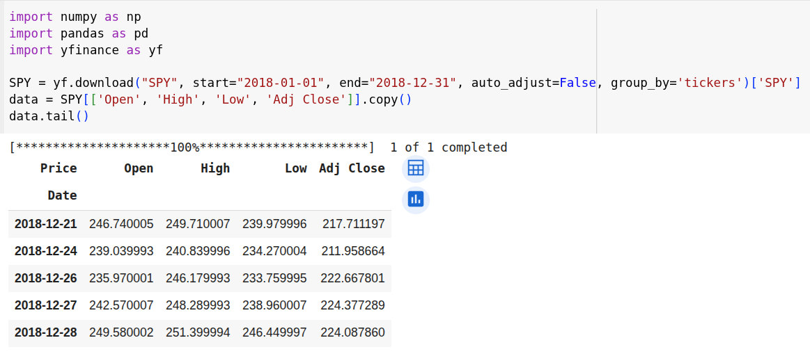
The first thing is to identify the states we want to model and analyze. In this example, we will simply consider whether the price moves up, down or is unchanged.
To summarize, our three possible states are:
- Up: The price has increased today from yesterday's price.
- Down: the price is decreased today compared to yesterday's price
- Flat: The price remains unchanged from the previous day.
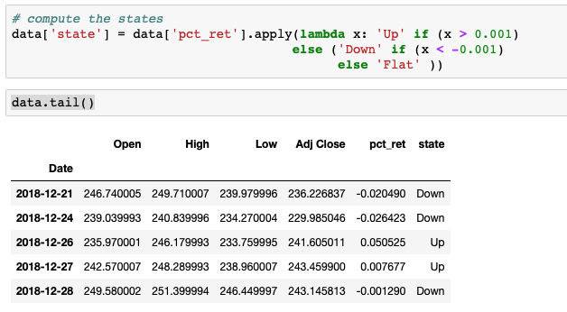
To obtain the states in our data frame, the first task is to calculate the daily return, although it should be remembered that the logarithmic return is usually better fitted to a normal distribution.

We then identify the possible states according to the return. The Flat state could be defined as a range and hence to consider an up/down as a minimum movement.
We are interested in analyzing the transitions in the prior day's price to today's price, so we need to add a new column with the prior state.

With the current state and the prior state, we can build the frequency distribution matrix.

Here we have gotten the frequency distribution of the transitions, which allows us to build the initial probability matrix or transition matrix at time t0.
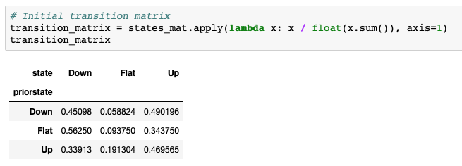
This would be our transition matrix in t0, we can build the Markov Chain by multiplying this transition matrix by itself to obtain the probability matrix in t1 which would allow us to make one-day forecasts.
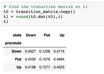
If we continue multiplying the transition matrix that we have obtained in t1 by the original transition matrix in t0, we obtain the probabilities in time t2.

Multiplying the transition matrix that we have obtained in t2 by the original transition matrix in t0, we obtain the probabilities in time t3 and so on until we find the equilibrium matrix where the probabilities do not change and therefore we cannot continue evolving the prediction.

Interestingly, you can get out identical results by raising the initial transition matrix to ‘n’ days to obtain the same result.

To find out the equilibrium matrix we can iterate the process up to the probabilities don’t change more.

With this example, we have seen in a simplified way how a Markov Chain works although it is worth analyzing the different libraries that exist in Python to implement the Markov Chains.
What is the Hidden Markov Model?
The Hidden Markov Model (HMM) was introduced by Baum and Petrie [4] in 1966 and can be described as a Markov Chain that embeds another underlying hidden chain.
The mathematical development of an HMM can be studied in Rabiner's paper [6] and in the papers [5] and [7] it is studied how to use an HMM to make forecasts in the stock market.
In this blog, we explain in depth, the concept of Hidden Markov Chains and demonstrate how you can construct Hidden Markov Models.
Also, check out this article which talks about Monte Carlo methods, Markov Chain Monte Carlo (MCMC).
If you want to detect a Market Regime with the help of a hidden Markov Model then check out this EPAT Project.
What is the difference between the Markov Model and the Hidden Markov Model?
As we have seen a Markov Model is a collection of mathematical tools to build probabilistic models whose current state depends on the previous state.
This is the initial view of the Markov Chain that later extended to another set of models such as the HMM.
The HMM is an evolution of the Markov Chain to consider states that are not directly observable but affect the behaviour of the model.
So, we learnt about Markov Chains and the Hidden Markov Model (HMM). I'd really appreciate any comments you might have on this article in the comment section below. Do feel free to share the link of this article. I've also provided the Python code as a downloadable file below.
References:
- [1] Seneta, Eugene. (2006). Markov and the creation of Markov Chains.
- [2] A.A. Markov, Extension of the law of large numbers to dependent quantities (in Russian), Izvestiia Fiz.-Matem. Obsch. Kazan Univ., (2nd Ser.), 15(1906), pp. 135–156 pp.
- [3] A.A. Markov, The extension of the law of large numbers onto quantities depending on each other. Translation into English of [2].
- [4] Baum, Leonard E., and Ted Petrie. 1966. Statistical inference for probabilistic functions of finite state Markov chains. The Annals of Mathematical Statistics 37: 1554–63.
- [5] Nguyen, Nguyet. 2018. Hidden Markov Model for Stock Trading.
- [6] Rabiner, Lawrence R. 1989. Hidden Markov Models and Selected Applications in Speech Recognition.
- [7] Hassan, Rafiul and Nath, Baikunth. 2005. Stock Market Forecasting Using Hidden Markov Model: A New Approach.
Disclaimer: All data and information provided in this article are for informational purposes only. QuantInsti® makes no representations as to accuracy, completeness, currentness, suitability, or validity of any information in this article and will not be liable for any errors, omissions, or delays in this information or any losses, injuries, or damages arising from its display or use. All information is provided on an as-is basis.
File in the download: Markov Model working - Python Code
