By Chainika Thakar
One might often ponder the need to understand and learn Stock Market Maths.
- What is the need to learn Maths for stock markets?
- Where do I learn about the application of maths in the stock markets?
- What are the basics of stock market maths?
- Which are the concepts to concentrate on while learning stock market maths?
Many aim to learn algorithmic trading from a mathematical point of view. Various mathematical concepts, statistics, and econometrics play a vital role in giving your stock trading that edge in the stock market.
Here's a complete list of everything that we are covering about Stock Market maths in this blog:
- What is stock market math?
- An overview of algorithmic trading
- Why does Algorithmic Trading require math?
- When and How Mathematics became popular in trading: A historical tour
- Mathematical concepts for stock markets
- Descriptive statistics
- Probability Theory
- Linear Algebra
- Calculus
What is stock market maths?
In the stock market, the maths used includes the concepts and calculations used to analyse and understand stock market behaviour, assess investment opportunities, and manage risk. It includes a range of techniques and tools that investors and traders use to make informed decisions.
Moving ahead, let us find out more about algorithmic trading and its association with Mathematics.
An overview of algorithmic trading
Algorithmic trading uses computer algorithms to automate and execute trades at high speeds. It relies on quantitative data to make informed decisions, removing emotions from trading. Strategies include trend following, arbitrage, and market making. While it offers speed and efficiency, it also involves risks like technical failures and requires constant monitoring. Effective algo trading demands strong technical skills, access to real-time data, and adherence to market regulations.
For algo trading for beginners, it's important to start with the fundamentals, including understanding basic trading strategies and the tools required for automating trades. With a solid foundation, beginners can gradually progress into more advanced topics, optimizing their strategies for the ever-changing market conditions.
To equip yourself with the necessary skills for algorithmic trading, consider enrolling in algo trading courses. These courses provide comprehensive training on various strategies, technical analysis, and the implementation of algorithms, ensuring you are well-prepared to navigate the complexities of the trading landscape.
The video below provides an overview of statistical arbitrage trading at Quantra:
Also, here is a brief market making video which can be quickly explored:
Next, we will find out what algorithmic trading maths means.
What is algorithmic trading math?
Algorithmic trading maths refers to the mathematical models and techniques used in the design and implementation of algorithms that automate the trading of financial instruments. This field combines principles from mathematics, statistics, computer science, and finance to create systems that can execute trades at high speeds and frequencies with minimal human intervention. The primary goal is to manage risks by exploiting market inefficiencies.
But why does algorithmic trading require maths and what is the relevance of the same? Let us find out the answer to this question next.
Why does Algorithmic Trading require math?
Algorithmic trading requires math to effectively analyse and predict market movements. Techniques like financial time series analysis and regression help in understanding historical data and forecasting future trends. Mathematical models provide the foundation for machine learning algorithms, which identify patterns and make predictions based on historical data.
Risk management is another critical area where math is essential. Quantifying risk involves using models such as Value at Risk (VaR) and performing stress tests to understand potential losses. Optimisation techniques, often grounded in mathematical theories like Modern Portfolio Theory (MPT), are used to allocate assets in a way that balances risk and return.
Pricing and valuation of financial instruments, especially derivatives, rely heavily on mathematical models. Calculus and stochastic processes, for instance, are used in the Black-Scholes model for option pricing, which helps in determining the fair value of derivatives based on their underlying assets.
Execution algorithms, which determine the optimal way to execute trades to minimise market impact and costs, also depend on math. Models like VWAP (Volume Weighted Average Price) and TWAP (Time Weighted Average Price) use mathematical formulas to break large orders into smaller ones over time, ensuring better execution quality.
Moving ahead, we will find out how mathematics became so important in the trading domain.
When and How Mathematics became popular in trading: A historical tour
In 1967, Edward Thorp, a mathematics professor at the University of California, published "Beat the Market", claiming to have a foolproof method for stock market success based on his blackjack system. This strategy involved selling stocks and bonds at one price and repurchasing them at a lower price, leading Thorp to establish the successful hedge fund Princeton/Newport Partners. The strategy's popularity drew physicists to finance, significantly impacting Wall Street.
Now let us head to the Mathematical concepts for algorithmic trading which are the core of this article.
Mathematical Concepts for Stock Markets
Starting with the mathematical for stock trading, it is a must to mention that mathematical concepts play an important role in algorithmic trading. Let us take a look at the broad categories of different mathematical concepts here:
Descriptive Statistics
Let us walk through descriptive statistics, which summarize a given data set with brief descriptive coefficients. These can be a representation of either the whole or a sample from the population.

Measure of Central Tendency
Here, Mean, Median and Mode are the basic measures of central tendency. These are quite useful when it comes to taking out average value from a data set consisting of various values. Let us understand each measure one by one.
Mean
This one is the most used concept in the various fields concerning mathematics and in simple words, it is the average of the given dataset. Thus, if we take five numbers in a data set, say, 12, 13, 6, 7, 19, 21, the formula of the mean is
$$\frac{x_1 + x_2 +x_3 + .......x_n}{n}$$
which makes it:
(12 + 13 + 6 + 7 + 19 + 21)/6 = 13
Furthermore, the trader tries to initiate the trade on the basis of the mean (moving average) or moving average crossover.
Here, let us understand two types of moving averages based on the ranges (number of days) of the time period they are calculated in and the moving average crossover:
1. Faster moving average (Shorter time period): A faster moving average is the mean of a data set (stock prices) calculated over a short period of time, say past 20 days.
2. Slower moving average (Longer time period): A slower moving average is the one that is the mean of a data set (stock prices) calculated from a longer time period say 50 days. Now, a faster-moving average and a slower moving average also come to a position together where a “crossover” occurs.
“A crossover occurs when a faster-moving average (i.e., a shorter period moving average) crosses a slower moving average (i.e. a longer period moving average). In other words, this is when the shorter period moving average line crosses a longer period moving average line.” ⁽¹⁾
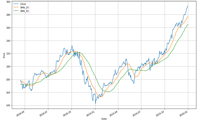
Here to explain it better, the graph image above shows three moving lines. The blue one shows the price line over the mentioned period. The green one indicates a slower-moving average of 50 days and the orange one indicates a faster-moving average of 20 days between April 2018 and January 2020.
Now starting with the green line, (slower moving average) the entire trend line shows the varying means of stock prices over longer time periods. The trend line follows a zig-zag pattern and there are different crossovers.
For example, there is a crossover between October 2018 and January 2019 where the orange line (faster-moving average) comes from above and crosses the green one (slower-moving average) while going down. This indicates that any individual or firm would be selling the stocks at this point since it shows a slump in the market. This crossover point is called the “meeting point”.
After the meeting point, ahead both the lines go down and then go up after a point to create one more (and then another) crossover(s). Since there are many crossovers in the graph, you should be able to identify each of them on your own now.
- Now, it is very important to note here that the “meeting point” is considered bullish if the faster-moving average crosses over the slower-moving average and goes beyond in the upward direction.
- On the contrary, it is considered bearish if the faster-moving average drops below the slower-moving average and goes beyond. This is so because in the former scenario, it shows that in a short time, there came an upward trend for particular stocks. Whereas, in the latter scenario it shows that in the past few days, there was a downward trend.
For example, we will be taking the same instances of the 20-day moving average for the faster-moving average and 50 days' moving average for the slower-moving average.
If the 20-day moving average goes up and crosses the 50-day moving average, it will show a bullish market since it indicates an upward trend in the past 20 days’ stocks. Whereas, if the 20-day moving average goes below the 50-day moving average, it will be bearish since it means that the stocks fell in the past 20 days.
In short, Mean is a statistical indicator used to estimate a company’s or even the market’s stock performance over a period of time. This period of time can be days, months and even years.
Going forward, the mean can also be computed with the help of an Excel sheet, with the following formula:
=Average(B2: B6)

Let us understand what we have done in the image above. The image shows the stock cap of different companies belonging to an industry over a period of time (can be days, months, or years).
Now, to get the moving average (mean) of this industry in this particular time period, we need the formula =(Average(B2: B6)) to be applied against the “Mean stock price”. This formula gives the command to Excel to average out the stock prices of all the companies mentioned from rows B2 to B6.
As we apply this formula and press “Enter” we get the result 330. This is one of the simplest methods to compute the Mean. Let us see how to compute the same in Python code ahead.
For further use, in all the concepts, let us assume values on the basis of Apple’s (AAPL) data set. In order to keep it universal, we have taken the daily stock price data of Apple, Inc. from Dec 26, 2022, to Dec 26, 2023. You can download historical data from Yahoo Finance.
yfinance is a useful library in Python with which you can download historical financial market data with sheer ease. Now, for downloading the Apple closing price data, we will use the following for all Python-based calculations ahead and yfinance will be mentioned.
In python, for taking out the mean of closing prices, the code will be as follows:
The Output is: 170.63337878417968
Ahead we will see how the Median differs from the Mean and how to compute it.
Median
Sometimes, the data set values can have a few values which are at extreme ends, and this might cause the mean of the data set to portray an incorrect picture. Thus, we use the median, which gives the middle value of the sorted data set. To find the median, you have to arrange the numbers in ascending order and then find the middle value. If the dataset contains an even number of values, you take the mean of the middle two values.
For example, if the list of numbers is: 12, 13, 6, 7, 19, then,
In ascending order, the numbers are: 6, 7, 12, 13, 19
Now, we know there are in total 5 numbers and the formula for the Median is:
(n+1)/2 value.
Hence, it will be n = 5 and
(5+1)/2 value will be 6/2= 3rd value.
Here, the 3rd value in the list is 12.
So, the median becomes 12 here.
Mainly, the advantage of the median is that, unlike the mean, it remains extremely valid in case of extreme values of data set which is the case in stocks. A median is required in case the average is to be calculated from a large data set, in which, the median shows an average which is a better representation of the data set.
For example, in case the data set is given as follows with values in INR:
75,000, 82,500, 60,000, 50,000, 1,00,000, 70,000 and 90,000.
Calculation of the median needs the prices to be first placed in ascending order, thus, prices in ascending order are:
50,000, 60,000, 70,000, 75,000, 82,500, 90,000, 1,00,000
Now, the calculation of the median will be:
As there are 7 items, the median is (7+1)/2 items, which makes it the 4th item. The 4th item in the ascending order is INR 75,000.
As you can see, INR 75,000 is a good representation of the data set, so this will be an ideal one.
In the financial world, where market prices vary time and again, the mean may not be able to represent the large values appropriately. Here, it was possible that the mean value would have not been able to represent the large data set. So, one needs to use the median to find the one value that represents the entire data set appropriately.
Excel sheet helps in the following way to compute the median:
=Median(B2:B6)

In the case of Median, in the image above, we have stock prices of different companies belonging to a particular industry over a period of time (can be days, months, or years). Here, to get the moving average (median) of the industry in this particular period, we have used the formula =Median(B2: B6). This formula gives the command to Excel to compute the median and as we input the same, we get the result 100.
The Python code here will be:
The Output is: 174.22782135009766
Great! Now as you have got a fair idea about Mean and Median, let us move to another method now.
Mode
Mode is a very simple concept since it takes into consideration that number in the data set which is repetitive and occurs the most. Also, the mode is known as a modal value, representing the highest count of occurrences in the group of data. It is also interesting to note that like mean and median, a mode is a value that represents the whole data set.
It is extremely imperative to note that, in some of the cases there is a possibility of there being more than one mode in a given data set. That data set which has two modes will be known as bimodal.
In the Excel sheet, the mode can be calculated as follows:
=Mode.SNGL(B1: B5)
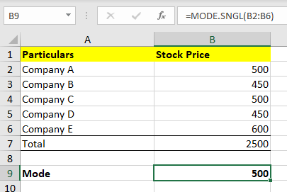
Similar to Mean and Median, Mode can also be calculated in the Excel sheet as shown in the image above. For example, you can put in the values of different companies in the Excel sheet and take out the Mode with the formula =Mode.SNGL(B1: B5).
(B1: B5) - represents the values from cell B1 to B5.
Now, if we take the closing prices of Apple from Dec 26, 2018, to Dec 26, 2019, we will find there is no repeating value, and hence the mode of closing prices does not exist because stock prices often change every day and rarely repeat exactly over a long period, especially with the inclusion of decimal values.
Also, there could be a stock that is not trading at all; in such cases, the price will remain constant, making it easy to identify the mode. Additionally, if you round stock prices to the nearest whole number, excluding decimal values, you are likely to find a mode as certain rounded prices will appear more frequently.
So when you try to calculate the Mode in Python with the following code:
It will throw the following error:
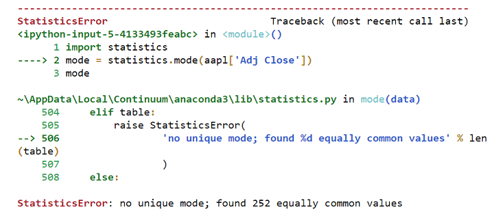
Hence, the mode does not make sense while observing closing price values.
Error in calculating mode
Hence, the mode does not make sense while observing closing price values. Coming to the significance of the mode, it is most helpful when you need to take out the repetitive stock price from the previous particular time period. This time period can be days, months and even years. Basically, the mode of the data will help you understand if the same stock price is expected to repeat in the future or not. Also, the mode is best utilised when you want to plot histograms and visualise the frequency distribution.
Amazing! This brings you to the end of the Measures of Central Tendency. Second, in the list of Descriptive Statistics is the Measure of Dispersion. Let us take a look at yet another interesting concept.
Measure of Dispersion
You will find the meaning of “Measure of Dispersion” right in its title since it displays how scattered the data is around the central point. It simply tells the variation of each data value from one another, which helps to give a representation of the distribution of the data. Also, it portrays the homogeneity and heterogeneity of the distribution of the observations.
In short, Measure of Dispersion shows how much the entire data varies from their average value.
The measure of dispersion can be divided into:
Now, let us understand the concept of each category.
Range
This is the most simple of all the measures of dispersion and is also easy to understand. Range simply implies the difference between two extreme observations or numbers of the data set.
For example, let X max and X min be two extreme observations or numbers. Here, Range will be the difference between the two of them.
Hence,
Range = X max - X min
It is also very important to note that Quant analysts keep a close follow up on ranges. This happens because the ranges determine the entry as well as exit points of trades. Not only the trades, but Range also helps the traders and investors in keeping a check on trading periods. This makes the investors and traders indulge in Range-bound Trading strategies, which simply imply following a particular trendline.
The trendlines are formed by:
- High-priced stocks (following an upper trendline) and
- Low-priced stocks (following a lower trendline)
In this the trader can purchase the security at the lower trendline and sell it at a higher trendline to earn profits. Hence, in Python, this simple code will be able to find the needed values for you:
The output is:
count    250.000000
mean     170.633379
std       18.099152
min      123.998451
25%      159.071522
50%      174.227821
75%      184.849152
max      197.589523
Name: Adj Close, dtype: float64
Let us take a look at how another measure, Quartile Deviation functions.
Quartile Deviation
This is the type which divides a data set into quarters. It consists of First Quartile as Q1, Second Quartile as Q2 and Third Quartile as Q3.
Here,
Q1 - is the number that comes between the smallest and the median of the data (1/4th) or the top 25%
Q2 - is the median of the data or
Q3 - is the number that comes between the median of data and the largest number (3/4th) or lower 25%
n - is the total number of values
The formula for Quartile deviation is: Q = ½ * (Q3 - Q1)
Since,
Q1 is top 25%, the formula for Q1 is - ¼ (n+1)
Q3 is also 25%, but the lower one, so the formula is - ¾ (n+1)
Hence, Quartile deviation = ½ * [(¾ (n+1) - ¼ (n+1)]
The major advantage, as well as the disadvantage of using this formula, is that it uses half of the data to show the dispersion from the mean or average. You can use this type of measure of dispersion to study the dispersion of the observations that lie in the middle. This type of measure of dispersion helps you understand dispersion from the observed value and hence, differentiates between the large values in different Quarters.
In the financial world, when you have to study a large data set (stock prices) in different time periods and want to understand the dispersed value (prices) from an observed one (average-median), Quartile deviation can be used.
The Python code here is by assuming a series of 10 random numbers:
The output is:
123.99845123291016
159.0715217590332
174.22782135009766
184.84915161132812
197.5895233154297
25.777629852294922
Great, moving ahead Mean absolute deviation is yet another measure which is explained ahead.
Mean Absolute Deviation
This type of dispersion is the arithmetic mean of the deviations between the numbers in a given data set from their mean or median (average).
Hence, the formula of Mean Absolute Deviation is:
(D0 + D1 + D2 + D3 + D4 ….Dn)/ n
Here,
n = Total number of deviations in the data set and
D0, D1, D2, and D3 are the deviations of each value from the average or median or mean in the data set and
Dn means the end value in the data set.
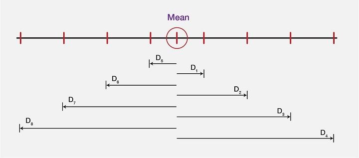
Explaining the Mean deviation, we will take a look at the image below, which shows a “computed mean” of a data set and the difference between each value (in the dataset) from the mean value. These differences or the deviations are shown as D0, D1, D2, and D3, …..D7.
For an instance, if the mean values are as follows:

Then, the Mean here will be calculated using the mean formula:
3 + 6 + 6 + 7 + 8 + 11 + 15 + 16 / 8 = 9
As the mean comes out to be 9, next step is to find the deviation of each data value from the Mean value. So, let us compute the deviations, or let us subtract 9 from each value to find D0, D1, D2, D3, D4, D5, D6, D7, and D8, which gives us the values as such:

As we are now clear about all the deviations, let us see the mean value and all the deviations in the form of an image to get even more clarity on the same:
Hence, from a large data set, the mean deviation represents the required values from observed data value accurately.
In python code, the computation of Mean deviation is as follows:
The output is 14.578809689453127
It is important to note that Mean deviation helps with a large dataset with various values which is especially the case in the stock market.
Going ahead, variance is a related concept and is further explained.
Variance
Variance is a dispersion measure which suggests the average of differences from the mean, in a similar manner as Mean Deviation does, but here the deviations are squared.
So,
$$Variance = [(DO)^2 + (D1)^2 + (D2)^2 + (D3)^2]/N$$
Here,
N = number of values in data set and
D0, D1, D2, D3 are the deviation of each value in the data set from the mean.
Here, taking the values from the example above, we simply square each deviation and then divide the sum of deviated values by the total number in the following manner:
$$(3)^2 + (6)^2 + (7)^2 + (8)^2 + (11)^2 + (15)^2 + (16)^2/8 = 99.5$$
In python code, it is as follows:
The output is 326.26900384104425
Let us jump to another measure called Standard Deviation now.
Standard Deviation
In simple words, the standard deviation is a calculation of the spread out of numbers in a data set. The symbol (sigma)represents Standard deviation and the formula is:
$$σ = \sqrt{Variance}$$
The formula of standard deviation is:
$$ σ = \sqrt{\frac{1}{N} \sum_{i=1}^N (x_i - μ)^2$$
Here, let us take the same values as in the two examples above and calculate Variance. Hence,
$$σ = \sqrt{99.5} = 9.97$$
Further, in Python code, the standard deviation can be computed as follows:
The output is: 18.062917921560853
All the types of measure of deviation bring out the required value from the observed one in a data set so as to give you the perfect insight into different values of a variable, which can be price, time, etc. It is important to note that Mean absolute data, Variance and Standard Deviation, all help in differentiating the values from average in a given large data set.
Visualisation
Visualisation helps the analysts to decide based on organised data distribution. There are four such types of Visualisation approach, which are:
Histogram

Age groups
Here, in the image above, you can see the histogram with random data on x-axis (Age groups) and y-axis (Frequency). Since it looks at a large data in a summarised manner, it is mainly used for describing a single variable.
For an example, x-axis represents Age groups from 0 to 100 and y-axis represents the Frequency of catching up with routine eye check up between different Age groups. The histogram representation shows that between the age group 40 and 50, frequency of people showing up was highest.
Since histogram can be used for only a single variable, let us move on and see how bar chart differs.
Bar chart
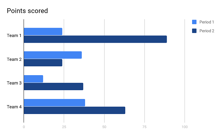
In the image above, you can see the bar chart. This type of visualization helps you to analyse the variable value over a period of time.
For an example, the number of sales in different years of different teams. You can see that the bar chart above shows two years shown as Period 1 and Period 2.
- In Period 1 (first year), Team 2 and Team 4 scored almost the same points in terms of number of sales. And, Team 1 was decently scoring but Team 3 scored the least.
- In Period 2 (second year), Team 1 outperformed all the other teams and scored the maximum, although, Team 4 also scored decently well just after Team 1. Comparatively, Team 3 scored decently well, whereas, Team 2 scored the least.
Since this visual representation can take into consideration more than one variable and different periods in time, bar chart is quite helpful while representing a large data with various variables.
Let us now see ahead how Pie chart is useful in showing values in a data set.
Pie Chart
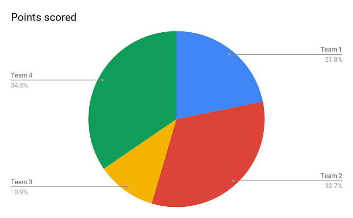
Above is the image of a Pie chart, and this representation helps you to present the percentage of each variable from the total data set. Whenever you have a data set in percentage form and you need to present it in a way that it shows different performances of different teams, this is the apt one.
For an example, in the Pie chart above, it is clearly visible that Team 2 and Team 4 have similar performance without even having to look at the actual numbers. Both the teams have outperformed the rest. Also, it shows that Team 1 did better than Team 3. Since it is so visually presentable, a Pie chart helps you in drawing an apt conclusion.
Moving further, the last in the series is a Line chart.
Line chart
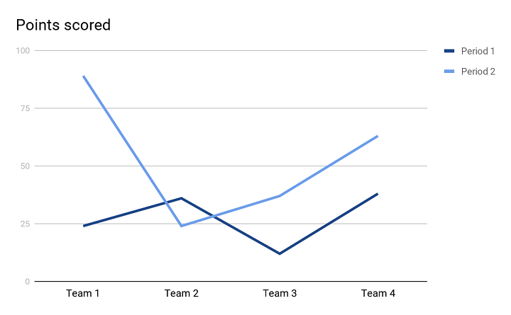
With this kind of representation, the relationship between two variables is clearer with the help of both y-axis and x-axis. This type also helps you to find trends between the mentioned variables.
In the Line chart above, there are two trend lines forming the visual representation of 4 different teams in two Periods (or two years). Both the trend lines are helping us be clear about the performance of different teams in two years and it is easier to compare the performance of two consecutive years. It clearly shows that in Period, 1 Team 2 and Team 4 performed well. Whereas, in Period 2, Team 1 outperformed the rest.
Okay, as we have a better understanding of Descriptive Statistics, we can move on to other mathematical concepts, their formulas as well as applications in algorithmic trading.
Probability Theory
Now let us go back in time and recall the example of finding probabilities of a dice roll. This is one finding that we all have studied. Given the numbers on dice i.e. 1,2,3,4,5, and 6, the probability of rolling a 1 is 1 out of 6 or ⅙. Such a probability is known as discrete in which there are a fixed number of results.
Now, similarly, the probability of rolling a 2 is 1 out of 6, the probability of rolling a 3 is also 1 out of 6, and so on. A probability distribution is the list of all outcomes of a given event and it works with a limited set of outcomes in the way it is mentioned above. But, in case the outcomes are large, functions are to be used.
If the probability is discrete, we call the function a probability mass function. In the case of a dice roll, it will be:
P(x) = 1/6 where x = {1,2,3,4,5,6}
For discrete probabilities, there are certain cases which are so extensively studied, that their probability distribution has become standardised. Let’s take, for example, Bernoulli's distribution, which takes into account the probability of getting heads or tails when we toss a coin.
We write its probability function as px (1 – p)(1 – x). Here x is the outcome, which could be written as heads = 0 and tails = 1.
Now, let us look into the Monte Carlo Simulation to understand how it approaches the possibilities in the future, taking a historical approach.
Monte Carlo Simulation
It is said that the Monte Carlo method is a stochastic one (in which there is sampling of random inputs) to solve a statistical problem. Well simply speaking, Monte Carlo simulation believes in obtaining a distribution of results of any statistical problem or data by sampling a large number of inputs over and over again. Also, it says that this way we can outperform the market without any risk.
One example of Monte Carlo simulation is rolling a dice several million times to get the representative distribution of results or possible outcomes. With so many possible outcomes, it would be nearly impossible to go wrong with the prediction of actual outcomes in future. Ideally, these tests are to be run efficiently and quickly which is what validates Monte Carlo simulation.
Although asset prices do not work by rolling a dice, they also resemble a random walk. Let us learn about Random Walk now.
Random walk
Random walk suggests that the changes in stock prices have the same distribution and are independent of each other. Hence, based on the past trend of a stock price, future prices can not be predicted. Also, it believes that it is impossible to outperform the market without bearing some amount of risk. Coming back to the Monte Carlo simulation, it validates its own theory by considering a wide range of possibilities and on the assumption that it helps reduce uncertainty.
Monte Carlo says that the problem is when only one roll of dice or a probable outcome or a few more are taken into consideration. Hence, the solution is to compare multiple future possibilities and customise the model of assets and portfolios accordingly.
After the Monte Carlo simulation, it is also important to understand Bayes’ theorem since it looks into the future probabilities based on some relatable past occurrences and hence, has usability. In simple words, Bayes’ theorem displays the possibility of the occurrence of an event based on past conditions that might have led to a relatable event to take place.
For example, say a particular age group between 50-55 had recorded maximum arthritis cases in months of December and January last year and last to last year also. Then it will be assumed that this year as well in the same months, the same age group may be diagnosed with arthritis.
This can be applied in probability theory, wherein, based on past occurrences with regard to stock prices, future ones can be predicted.
There is yet another one of the most important concepts of Mathematics, known as Linear Algebra which now we will learn about.
Linear Algebra
Let's learn about Linear Algebra in brief.
What is linear algebra?
In simple words, linear algebra is the branch of mathematics that consists of linear equations, such as a1 x1 + ……. + an xn = b. The most important thing to note here is that Linear algebra is the mathematics of data, wherein, Matrices and Vectors are the core of data.
What are matrices?
A matrix or matrices is an accumulation of numbers arranged in a particular number of rows and columns. Numbers included in a matrix can be real or complex numbers or both.
For example, M is a 3 by 3 matrix with the following numbers:
0 1 3
4 5 6
2 4 7
What are the vectors?
In simple words, Vector is that concept of linear algebra that has both, a direction and a magnitude.
For example, \( \mathbf{V} \) is:
\[ \mathbf{V} = \begin{bmatrix} 9 \\ 6 \\ -5 \end{bmatrix} \]
Now, If X =
$$[X_1]$$
$$[X_2]$$
$$[X_3]$$
Then,
MX = V which will become ,
$$[0+X_2+3X_3] = [9]$$
$$[4X_1+5X_2+6X_3] = [6]\; and$$
$$[2X_1+4X_2+7X_3] = [-5]$$
In this arrow, the point of the arrowhead shows the direction and the length of the same is magnitude.
Above examples must have given you a fair idea about linear algebra being all about linear combinations. These combinations make use of columns of numbers called vectors and arrays of numbers known as matrices, which concludes in creating new columns as well as arrays of numbers. There is a known involvement of linear algebra in making algorithms or in computations. Hence, linear algebra has been optimized to meet the requirements of programming languages.
Also, for improving efficiency, certain linear algebra implementations (BLAS and LAPACK) configure the algorithms in an automated manner. This helps the programmers to adapt to the specific nature of the computer system, like cache size, number of cores and so on.
In python code :
The output is:
rank of A: 3
Trace of A: 12
Determinant of A: 2.0000000000000004

Inverse of A: [[ 5.5  2.5 -4.5]
 [-8.  -3.   6. ]
 [ 3.   1.  -2. ]]

Matrix A raised to power 3:
 [[ 122  203  321]
 [ 380  633 1002]
 [ 358  596  943]]
Let us move ahead to another known concept used in algorithmic trading called Linear Regression.
Linear Regression
Linear Regression is yet another topic that helps in creating algorithms and is a model which was originally developed in statistics. Linear Regression is an approach for modelling the relationship between a scalar dependent variable y and one or more explanatory variables (or independent variables) denoted x.
Nevertheless, despite being a statistical model, it helps as the machine learning regression algorithm to predict prices by showing the relationship between input and output numerical variables.
How is Machine Learning helpful in creating algorithms?
Machine learning implies an initial manual intervention for feeding the machine with programs for performing tasks followed by an automatic situation-based improvement that the system itself works on. In short, Machine learning with its systematic approach to predict future events helps create algorithms for successful automated trading.
Calculating Linear Regression
The basic formula of Linear Regression is: Y = mx+b
Below, you will see the representations of x & y clearly in the graph:
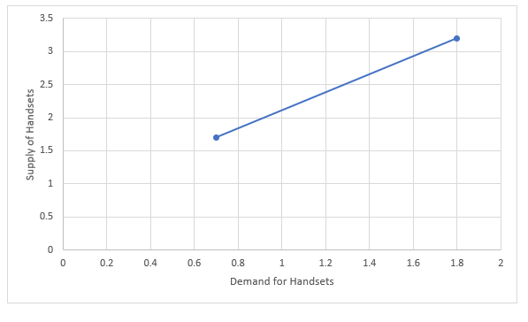
In the graph above, the x-axis and y-axis both show variables (x and y). Since more sales of handsets or demand (x-axis) of handsets are provoking a rise in supply (y-axis) of the same, a steep line is formed. Hence, to meet this rising demand, the supply or the number of handsets also rises.
Simply,
y = how much the trend line goes up (Supply)
x = how far the trend line goes (Demand)
b = intercept of y (where the line crosses the y-axis)
In linear regression [²], the number of input values (x) are combined to produce the predicted output values (y) for that set of input values. Both the input values and output values are numeric.
Using machine learning regression for trading is explained briefly in this video below:
As we move ahead, let us take a look at another concept called Calculus which is also imperative for algorithmic trading.
Calculus
Calculus is one of the main concepts in algorithmic trading and was actually termed infinitesimal calculus, which means the study of values that are really small to be even measured. In general, Calculus is a study of continuous change and hence, very important for stock markets as they keep undergoing frequent changes.
Coming to the types of calculus, there are two broad terms:
- Differential Calculus: It calculates the instantaneous change in rates and the slopes of curves.
- Integral Calculus: This one calculates the quantities summed up together.
In Calculus, we usually calculate the distance (d) in a particular time period(t) as:
\( d = at^2 \)
where,
\( d \) is distance,
\( a \) is acceleration, and
\( t \) is time
Now, to simplify this calculation, let us suppose \( a = 5 \).
\( d = 5t^2 \)
Now, if time (\( t \)) is 1 second and distance covered is to be calculated in this time period which is 1 second, then,
\( d = 5(1)^2 = 5 \, \text{metres/second} \)
Here, it shows that the distance covered in 1 second is 5 metres. But, if you want to find the speed at which 1 second was covered(current speed), then you will need a change in time, which will be t. Now, as it is really less to be counted, t+t will denote o second.
Let us calculate the speed between t and t seconds as we know from the previous calculation that at 1 second, the distance covered was 5m/s. Now, with the same formula, we will also find the distance covered at 0 seconds (t +t ):
So, \( d = 5t^2 \)
\( d = 5(t + t)^2 \)
\( d = 5(1 + t)^2 \, \text{m} \)
Expanding \( (1 + t)^2 \), we will get \( 1 + 2t + t^2 \)
\( d = 5(1 + 2t + t^2) \, \text{m} \)
\( d = 5 + 10t + 5t^2 \, \text{m} \)
Since, \( \text{Speed} = \frac{\text{distance}}{\text{time}} \)
\( \text{speed} = \frac{5 + 10t + 5t^2 \, \text{m}}{t \, \text{s}} \)
This brings us to the conclusion, \( 10 + 5t \, \text{m/s} \)
Since t is considered to be a smaller value than 1 second, and the speed is to be calculated at less than a second (current speed), the value of t will be close to zero.
Therefore, the current speed = 10m/s
This study of continuous change can be appropriately used with linear algebra and also can be utilised in probability theory. In linear algebra, it can be used to find the linear approximation for a set of values. In probability theory, it can determine the possibility of a continuous random variable. Being a part of normal distribution calculus can be used to find out normal distribution.
Awesome! This brings us to the end of all the essential mathematical concepts required for Quants/HFT/Algorithmic Trading.
Conclusion
In this blog, we explored the essential role of mathematics in the stock market, starting with basic stock market maths and algorithmic trading. We covered why mathematics is vital for trading algorithms, followed by a historical perspective on its rise in finance. Learn more about the stock market through our stock market beginner course.
Key mathematical concepts such as descriptive statistics, data visualisation, probability theory, and linear algebra were discussed. We also highlighted linear regression, its calculations, and the importance of machine learning in algorithm creation.
Lastly, we touched upon the relevance of calculus in financial modelling. This guide provides a comprehensive overview of how maths drives successful stock market trading and algorithm development.
In case you are also interested in developing lifelong skills that will always assist you in improving your trading strategies. In this algorithmic trading course, you will be trained in statistics & econometrics, programming, machine learning and quantitative trading methods, so you are proficient in every skill necessary to excel in quantitative & algorithmic trading. Learn more about the EPAT course now!
Note: The original post has been revamped on 21st February 2024 for recentness, and accuracy.
Disclaimer: All data and information provided in this article are for informational purposes only. QuantInsti® makes no representations as to accuracy, completeness, currentness, suitability, or validity of any information in this article and will not be liable for any errors, omissions, or delays in this information or any losses, injuries, or damages arising from its display or use. All information is provided on an as-is basis.