By Vibhu Singh and Mandeep Kaur
In this blog, we will discuss various aspects of the portfolio evaluation and portfolio measurement. We’ll start discussing with why evaluation and measurement are necessary and will then move on to how to compute and analyze the returns generated by the portfolio after a particular time period.
One key difference between the calculation of portfolio returns in the previous blog and this blog is that, here, we will see how to compute the returns after they are generated. In the previous case, we were computing expected returns of the portfolio based on the expected returns of the constituent stocks.
This article covers:
- Why Performance Measurement and Evaluation is required?
- Calculation of Portfolio Returns
- Time-Weighted Rate of Return (TWRR)
- Money-Weighted Rate of Return (MWRR)
- Computing TWRR in Python
- Computing MWRR in Python
- Portfolio Return Components
- Performance Attribution
- Summary
Why Performance Measurement and Evaluation is required?
Evaluation of the performance measurement is necessary for investors and portfolio managers both. However, the need for evaluating may be different for these two sets of people.
Performance evaluation also shows the areas of effectiveness as well as improvements in the investment scheme.
Some of the benefits for evaluating the portfolio performance include the following
- The return performance of the investment over time (performance measurement)
- How the observed performance is attained (performance attribution)
- If the performance is due to investment decisions (performance appraisal)
Calculation of Portfolio Returns
Let us assume that:
the period of evaluation is t,
market value at the start of the time period was MV0 and
at the end of this time period is MVt.
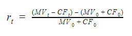
Further, the cash inflows at the start and end of the time period t are CF0 and CFt.
The return from the portfolio for this period can be computed as:
Consider the example below.
On Jan 1, 2017, the value of the portfolio was $ 100,000 and another $ 50,000 was inducted in the portfolio. There were no intermediate cash flows and on Dec 31, 2017, another $ 25,000 were introduced.
The portfolio value as on close of business on Dec 31, 2017, is $ 200,000. The time period here is 1 year.
The return from the portfolio can be computed in python as shown.
The return from the portfolio is: 16.67
As we can see from the above equation, we add any external cash inflow at the beginning of the period to the initial market value of the portfolio and subtract any external cash inflow at the end from the market value at time period t.
The only assumption made here is that no liquid cash is maintained with the portfolio manager and all the cash is invested in the portfolio.
Now let’s assume that there are multiple such time periods or multiple cash inflows within the time period for which we are computing the returns.
In these cases, we use time-weighted rate of return (TWRR) and money-weighted rate of return (MWRR) respectively.
Time-Weighted Rate of Return (TWRR)
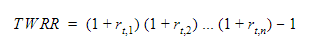
If there are n time periods within our analysis period t and rt,i denotes the return from the sub-period i, then the time-weighted rate of return can be computed as:
Money-Weighted Rate of Return (MWRR)
MWRR is essentially the internal rate of return from the portfolio. While computing the IRR, the initial market value MV0 is considered as the cash inflow at t = 0. All the current inflows are considered as positive in the below equation.
Let R be the internal rate of return or the MWRR from the portfolio, it can be computed using the equation:
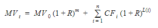
Where,
MVt is the ending market value of the portfolio
MV0 is the initial market value
m is the number of time units in the considered period (number of days, weeks, months, etc.)
CFi are the clash flows
L(i) is the time units remaining after the cash flow CFi is inducted
Using this method, we will now compute the TWRR and MWRR for the given portfolio.
- Market value as on start of Jan 1 2017: $ 100,000
- Market value as on close of Mar 31 2017: $ 110,000
- Cash inflow on Apr 1 2017: $ 5,000
- Market value as on close of Jun 30 2017: $ 120,000
- Market value as on close of Sep 30 2017: $ 125,000
- Cash inflow on Dec 31 2017: $ 7,000
- Market value as on close of Dec 31 2017: $ 140,000
Calculating TWRR in Python
The TWRR for the portfolio is (in %age): 27.22
Calculating MWRR in Python
This computation is very easy. You just need the numpy_financial library! See below:
The MWRR for the portfolio is (in %age): 24.65
Portfolio Return Components
Having calculated the return from the portfolio, we will analyze various components of the return. These returns can be divided into three components.
P = M + S + A
Where,
P is the return from the portfolio
M is the market return
S = B - M
Where,
B is the benchmark return
S signifies excess return due to investing style (for example, a manager investing only in large-cap automotive sector)
A = P - B, is the active return generated by the manager over the benchmark
Performance Attribution
The active return or the value-added return (return of the portfolio - benchmark return) can be attributed or broken into three components.
- Pure sector selection: Pure sector selection assumes that the manager holds the same sectors in the portfolio as in the benchmark but in different proportions. The proportion of each security within each sector is also held the same as in the benchmark. The active performance is due to the selection of the weights of the sector only.
- Within-sector selection return: This assumes that the portfolio manager holds all the sectors in the same proportion as the benchmark and the returns are generated by adjusting the weights of securities in each sector.
- Allocation/selection interaction return: This involves the joint effect of changing the weights of both the securities and the sectors in the portfolio. Any increase in the weight of a security will also increase the weight of that sector.

Where,
RV = Value added return
wP, j = Portfolio weight of sector j
wB, j = Benchmark weight of sector j
RP, j = Portfolio return of sector j
RB, j = Benchmark return of sector j
RB = Return of portfolio’s benchmark
S = Number of sectors
In the above equation, the first term refers to the pure sector allocation, the second term refers to the selection interaction return while the third term refers to the within-sector selection return.
We will now compute all the three components of active return for the below portfolio using python.
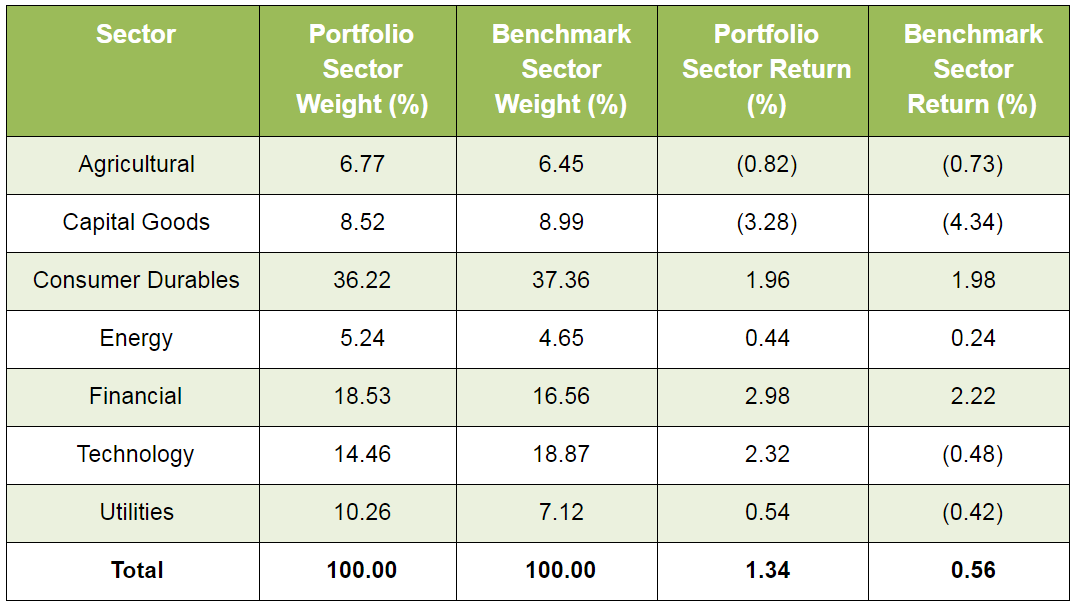
The sum of portfolio weights is:  100
The sum of benchmark weights is:  100
The return from the portfolio is:  1.34
The return from the benchmark is:  0.56
The active return is:  0.78
The pure selection return is:  0.05
The selection interaction return is:  -0.08
The within-sector selection return is:  0.81
The total active return from the components is:  0.78
As can be seen from the above results that the sum of all the three components add-up to the active returns from the portfolio (also known as alpha).
Summary
In this blog, we saw how to compute the returns from a portfolio in a given time period with multiple cash flows using TWRR and MWRR.
We also saw how to divide the portfolio returns into components. Lastly, we covered the attribution of active return into three components, viz., pure sector allocation, within-sector allocation and allocation/selection interaction returns.
If you're a portfolio manager or a quant who wishes to construct their portfolio quantitatively, generate returns and manage risks effectively can check out the course on Portfolio Management on Quantra.
File in the download
- Portfolio Analysis - Performance, Measurement and Evaluation – Python Code
Disclaimer: All investments and trading in the stock market involve risk. Any decisions to place trades in the financial markets, including trading in stock or options or other financial instruments is a personal decision that should only be made after thorough research, including a personal risk and financial assessment and the engagement of professional assistance to the extent you believe necessary. The trading strategies or related information mentioned in this article is for informational purposes only.