By Ajay Pawar
Have you ever noticed how a model that once predicted stock prices with pinpoint accuracy suddenly starts missing the mark? This isn’t just bad luck—it’s often the result of concept drift or model drift, common challenges in the ever-evolving world of quantitative finance. Financial markets are anything but static; their dynamic nature means yesterday’s data patterns might not hold true today.
That’s where Walk-Forward Optimization (WFO) comes into play. By continuously retraining your model on the most recent data, WFO helps maintain predictive accuracy even as market conditions shift. In this guide, you’ll learn how to implement WFO in Python, using XGBoost for stock price prediction.
Pre-requisite blogs:
This blog is the second installment in the Walk-Forward Optimization (WFO) series. To fully understand the concepts discussed here, it is recommended that you first go through the Introduction to Walk-Forward Optimization, which lays the foundation for applying WFO in trading models.
Additionally, to further strengthen your grasp on machine learning techniques, Machine Learning Logistic Regression in Python introduces logistic regression and its applications in financial markets. Since data quality plays a crucial role in building reliable trading models, Data Preprocessing covers essential steps to clean and prepare datasets. Moreover, understanding Autocorrelation in Trading will help you analyze dependencies within time series data, a key factor in financial modeling.
The blog covers:
Objective of This Article
By the conclusion of this article, you will acquire:
- Technical Proficiency in WFO Implementation: Learn to structure your machine learning workflow to incorporate WFO for time-series forecasting.
- Critical Steps and Best Practices: Understand the nuances of applying WFO in financial modeling, from data preprocessing to model evaluation.
- Application with XGBoost: Utilize XGBoost, a highly efficient gradient boosting algorithm, optimized for speed and performance in financial datasets.
Who Should Read This Article?
This guide is tailored for:
- Data Scientists specializing in time-series forecasting.
- Quantitative Analysts aiming to enhance predictive models for financial markets.
- Algorithmic Traders and Portfolio Managers looking to integrate adaptive machine learning techniques into trading strategies.
Why Do We Need Walk-Forward Optimization?
In quantitative finance, model performance degradation over time is a common challenge, often attributed to:
- Concept Drift occurs when the underlying relationships between input features and target variables evolve over time. For instance, economic indicators influencing stock prices today may not have the same impact in the future due to changing market conditions or policies.
- Model Drift, on the other hand, refers to the decline in predictive accuracy caused by shifts in data distribution or outdated models that no longer capture current market dynamics.
Both issues highlight the non-stationary nature of financial markets, where static models struggle to maintain accuracy over time. This is where Walk-Forward Optimization (WFO) becomes essential, offering a robust framework to continually retrain models on the most recent data, effectively addressing these drifts and maintaining high predictive performance.
Key Advantages of WFO in Algorithmic Trading
- Mitigating Overfitting: Regular retraining prevents overfitting to outdated market conditions, ensuring the model generalizes well to new data.
- Enhancing Predictive Robustness: By constantly updating the model, WFO captures the evolving relationships in financial time-series data.
- Simulating Live Trading Environments: WFO mirrors real-world algorithmic trading, where models must adapt to continuously streaming data, making it essential for live trading systems and automated portfolio management.
For a foundational understanding of Walk-Forward Optimization, refer to this comprehensive guide on WFO.
Why XGBoost for Financial Modeling?
XGBoost (Extreme Gradient Boosting) is a powerful machine learning algorithm known for its scalability and superior performance on structured data. In quantitative finance, it is extensively used for predicting stock prices, risk modeling, and portfolio optimization due to its:
- Handling of Missing Data: Automatically manages missing values in time-series data.
- Regularization Techniques: Incorporates L1 and L2 regularization to reduce overfitting.
- Parallel Processing: Enhances computational efficiency, crucial for large-scale financial datasets.
For an in-depth understanding of XGBoost and its applications in financial forecasting, refer to Forecasting Markets Using XGBoost
Let's dive into the technical implementation of Walk-Forward Optimization step-by-step!
Python Script: Walk-Forward Optimization with XGBoost
What We’re About to Do:
We’ll begin by collecting historical stock data and preparing it for analysis. This involves cleaning the data, removing unnecessary columns like volume, formatting dates correctly, and rounding price data for consistency. We will add features like RSI to enhance the model’s predictive power. Additionally, we’ll create lagged features that use past price data to predict future prices, mimicking how traders analyse historical trends to forecast movements.
The core of WFO lies in iteratively training and updating the model. Starting from a specific date, we’ll move through the dataset day by day. For each day, the model is trained on data up to that point, and a prediction is made for the next day’s price. After a set number of days (our retraining interval), the model is retrained using the latest data to ensure it adapts to new market trends. This continuous retraining helps the model stay relevant in the face of evolving market dynamics.
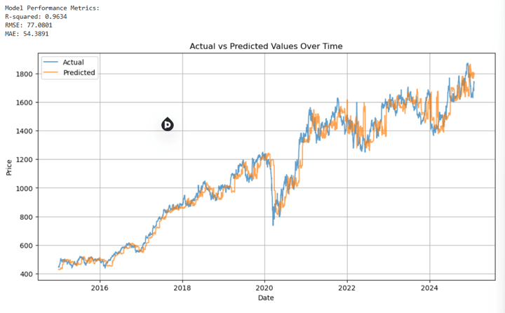
Then XGBoost model will be trained on features scaled to a uniform range, helping it converge faster and perform more accurately. As the model walks forward through time, it generates predictions for each new day. We’ll then compare these predictions to actual stock prices to evaluate performance using metrics like R-squared (R²).
Finally, we’ll visualise the predicted stock prices against the actual prices to assess the model’s performance over time.
Importing Essential Libraries
We begin by pulling in all the libraries essential for data handling, model building, and visualisation:
Configuring Parameters
These parameters shape how the analysis unfolds, defining data sources, timeframes, and model behaviour:
- TICKER: Stock symbol to analyse.
- START_DATE & WFO_START_DATE: Timeframe for data collection and prediction start.
- RETRAIN_PERIOD: How often the model is retrained to adapt to new market conditions.
- SLIDING_WINDOW: Focuses training on recent data trends.
- TRAIN_RATIO: Splits data into training and testing.
- LOOKBACK_PERIODS: Number of previous days used to create features.
- PREDICT_AHEAD: Number of days into the future to predict.
- TARGET_COLUMN: The price metric the model aims to forecast.
- RSI_PERIOD: Period for calculating the Relative Strength Index.
Data Download and Preparation
Download Historical Data:
- We fetch stock data (Open, High, Low, Close, Volume) from the specified start date (START_DATE) up to today.
- The parameter auto_adjust=True ensures that prices are adjusted for dividends and splits, giving a cleaner time-series.
Preprocessing:
- The script removes unneeded columns (e.g., Volume).
- We convert the index to a datetime format, which simplifies time-based operations.
- Rounding prices to three decimals and dropping rows with missing values helps maintain consistency. Adding the RSI Indicator
- RSI (Relative Strength Index) is computed using the rolling averages of gains and losses over a given period.
Once calculated, any rows with newly introduced missing values (e.g., due to rolling windows) are dropped.
Walk-Forward Setup:
- Initialise components like scalers and place holders like results and dataframe.
- Defining Start Date for WFO"
- We designate a start date for when we begin “walking forward” (WFO_START_DATE).
- If there is a sliding window (e.g., 200 days), we shift the start date to ensure there’s enough prior data for that window.
- Filtering the Dataset:
- We focus on rows starting from this WFO start date (or adjusted date if sliding is used).
- The remaining subset of dates is what we iterate over day by day.
Main Prediction Loop Explanation
This section walks through the main walk-forward prediction loop in a time-series forecasting model. It leverages historical data, creates lagged features, and retrains the model at defined intervals to make accurate predictions.
1. Iterate Through Each Date
The loop runs through each date in the filtered dataset (dates). This approach simulates how predictions would be made in real-world scenarios, processing one day at a time.
2. Data Selection: Historical Context
For each date, we collect all historical data up to that point. If using a sliding window, only the most recent N days are considered, allowing the model to focus on the most relevant data.
Sliding Window: Useful when older data becomes less relevant over time.
3. Feature Engineering: Lagged Features Creation
To capture historical patterns, we generate lagged versions of each feature (e.g., Close, Open, RSI). These lagged features provide context from previous days.
Lagging: Helps the model understand past behavior influencing future outcomes.
4. Saving the Most Recent Data Point
We store the last row of lagged features to make the next prediction.
5. Target Variable Creation (Future Price)
The target variable is the future price we aim to predict. We shift the target column forward by PREDICT_AHEAD days.
Purpose: Aligns the current data with the future price we want to forecast.
6. Data Cleaning: Removing Missing Values
Rows with missing values (from lagging or shifting) are removed to ensure clean data for model training.
7. Train/Test Split
The data is split chronologically to ensure the model trains on past data and tests on more recent data.
No Shuffling: Maintains the time order, critical for time-series forecasting.
8. Conditional Model Retraining
The model is retrained if it's the first iteration or when the retrain period is reached.
- Scaling: Ensures features are on the same scale for better model performance.
- XGBoost Regressor: A powerful model for regression tasks with great handling of time-series data.
- Performance Metrics: R² scores to evaluate how well the model fits the data.
9. Prediction on Latest Data
The model predicts the next price using the most recent lagged features.
10. Storing Results
Results for each iteration are stored in a temporary DataFrame and then appended to the main results.
Result Storage: Keeps track of predictions, retraining status, and model performance for evaluation.
Results Compilation and Evaluation
We align predictions with actual values, compute evaluation metrics and plot actual versus predicted stock prices.
Conclusion
In conclusion, this code offers a tangible roadmap for implementing Walk-Forward Optimization (WFO) in a real-world scenario. By incrementally retraining an XGBoost model, it tackles the inherent non-stationarity of financial time-series and provides a clear structure for experimenting with parameters like lookback periods, retraining frequencies, and predictive horizons. This end-to-end framework—from data acquisition and feature engineering to iterative model updating and performance evaluation—enables practitioners to adapt quickly to changing market conditions, making it a robust foundation for quantitative finance applications.
To elevate your WFO strategy, experiment with different algorithms—like classification models, neural networks, and ensemble methods. For a deeper dive into refining data preparation, check out Data and Feature Engineering for Trading.
After mastering WFO, transform your predictions into actionable trading signals and validate them through rigorous backtesting. This step helps you assess historical performance, revealing insights into potential profitability and risk. To sharpen your backtesting skills, explore Backtesting Trading Strategies and Backtesting Basics. If you're keen on backtesting machine learning strategies with less coding, Blueshift offers a hands-on, visual approach.
By leveraging these resources and continuously refining your approach, you’ll be well-equipped to navigate the dynamic financial markets and improve your trading performance.
Continue learning with these blogs:
It is time to explore more advanced techniques in machine learning, backtesting, and model validation.
If you are looking to implement machine learning models in trading, Machine Learning Strategy Using Blueshift offers a no-code approach to building and testing strategies in a visual programming environment.
Additionally, before deploying any model in live markets, backtesting is essential. The Backtesting: A Step-by-Step Guide explains how to test strategies effectively to ensure they perform well under real-world market conditions.
Cross-Validation for Model Testing
One of the key aspects of validating machine learning models in trading is cross-validation. If you want to prevent overfitting and improve the robustness of your models, Cross-Validation: Embargo, Purging & Combinatorial Approaches details methods to refine model performance.
Similarly, Cross-Validation for Machine Learning-Based Trading Models explores different validation techniques specifically tailored for financial data.
Structured Learning with Quantra
For a more structured and hands-on learning experience, Quantra offers various courses tailored to machine learning and backtesting.
If you are interested in classification models, Trading with Machine Learning: Classification & SVM is a great course to explore.
For traders looking to incorporate decision trees into their strategies, Decision Trees for Trading by Dr. Ernest Chan provides in-depth knowledge from a well-known quant expert.
Additionally, since feature selection plays a crucial role in model accuracy, Data and Feature Engineering for Trading teaches how to refine datasets for better predictive performance.
If you want to focus on backtesting, Backtesting Trading Strategies guides you through designing, testing, and improving your trading strategies efficiently.
For traders looking for a complete learning journey, Machine Learning & Deep Learning in Trading provides a structured learning track covering essential machine learning techniques, from basic models to deep learning applications in financial markets.
Backtesting with Blueshift
Blueshift – An all-in-one platform designed for research, backtesting, and algorithmic trading. Blueshift provides a fast, flexible, and reliable solution for testing strategies across various asset classes and trading styles.
File in the download:
- The Python code implementing the Walk-Forward Optimization (WFO) strategy using XGBoost is provided.
- You can download the Python .py file, install essential libraries, and run the code.
- Feel free to make changes to the code as per your comfort.
Disclaimer: All investments and trading in the stock market involve risk. Any decision to place trades in the financial markets, including trading in stock or options or other financial instruments is a personal decision that should only be made after thorough research, including a personal risk and financial assessment and the engagement of professional assistance to the extent you believe necessary. The trading strategies or related information mentioned in this article is for informational purposes only.