Introduction to XGBoost in Python

XGBoost…!!!! Often considered a miraculous tool embraced by machine learning enthusiasts and competition champions, XGBoost was designed to enhance computational speed and optimise machine learning model’s performance.

You must be wondering what will be the key areas you will tap into with this blog.

Well, you can see below some unique pointers we will be covering with this blog:

• How to unlock the predictive power of XGBoost: Learn how XGBoost harnesses high accuracy to predict market dynamics effectively.
• How to utilise ensemble learning: Discover how “ensemble learning” strengthens predictions while reducing overfitting risks.
• Navigation of regulatory terrain: Explore regulatory compliance strategies to ensure alignment with financial regulations.
• Efficiency & scalability insights: Understand how XGBoost's efficiency and scalability enhance trading strategies for various scales.
• Practical trading tips: Gain insights into practical data preprocessing and risk management techniques for successful trading.
• How to stay ahead with continuous learning: Embrace continuous learning to stay updated on evolving machine learning techniques and trading strategies.
• Collaboration can lead to success: Learn how collaboration with industry experts enriches trading insights and strategies.

Also, you will learn to figure out the strategy returns so that you can:

1. Assess the strength of your strategy
2. Optimise the strategy parameters for getting better returns

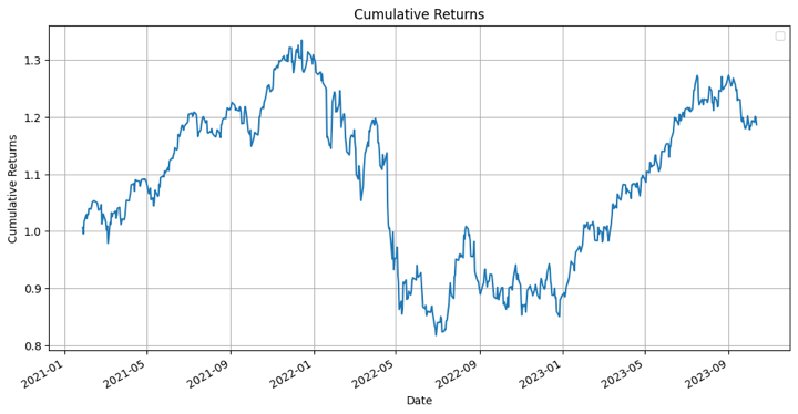
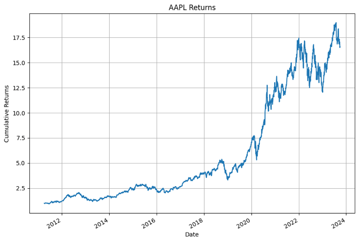
Cumulative returns graph from the strategy

Below you can see the cumulative returns of the strategy mentioned in this blog.

Now that you know what lies ahead, let's proceed!!!

We will cover the following things:

• Brief of XGBoost
• How did the need for XGBoost arise?
• Why is XGBoost better than other ML techniques?
• XGBoost fundamentals
• How to use the XGBoost model for trading?
• Pros of using XGBoost model in trading
• Challenges of using XGBoost model in trading
• Tips to overcome the challenges of XGBoost model

Brief of XGBoost

XGBoost, short for "eXtreme Gradient Boosting," is rooted in gradient boosting, and the name certainly has an exciting ring to it, almost like a high-performance sports car rather than a machine learning model.

However, its name perfectly aligns with its purpose – supercharging the performance of a standard gradient boosting model.

Tianqi Chen, the mastermind behind XGBoost, emphasised its effectiveness in managing overfitting through a more regulated model formulation, resulting in superior performance.

What is boosting or ensemble methods?

The sequential ensemble methods, also known as “boosting”, creates a sequence of models that attempts to correct the mistakes of the models before them in the sequence.

The first model is built on training data, the second model improves the first model, the third model improves the second, and so on.

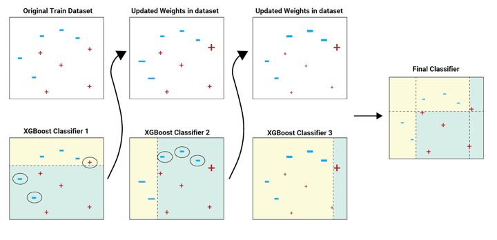
In the above image example, the train dataset is passed to the classifier 1.

The yellow background indicates that the classifier predicted hyphen, and the sea green background indicates that it predicted plus. The classifier 1 model incorrectly predicts two hyphens and one plus. These are highlighted with a circle.

The weights (as shown in the updated datasets) of these incorrectly predicted data points are increased (to a certain extent) and sent to the next classifier. That is to classifier 2.

The classifier 2 correctly predicts the two hyphens which classifier 1 was not able to predict. But classifier 2 also makes some other errors. This process continues and we have a combined final classifier which predicts all the data points correctly.

The classifier models can be added until all the items in the training dataset are predicted correctly or a maximum number of classifier models are added. The optimal maximum number of classifier models to train can be determined using hyperparameter tuning.

Example from a beginner’s perspective

Now, let us learn about this as a beginner who doesn’t know much about machine learning.

Sequential ensemble methods, known as "boosting," work like a team of learners. Each learner tries to fix the mistakes made by the previous one. Think of it as a relay race where the baton is improving with each handoff.

In the example, the first classifier gets the training data. It makes some mistakes (shown with yellow and blue backgrounds), and those mistakes get extra attention. The second classifier focuses on fixing those errors. This process continues until all data is correctly predicted or a limit on learners is reached. The right limit is chosen using hyperparameter tuning. It's like a team effort where each member makes the group better.

XGBoost is a special tool in machine learning that's exceptionally good at making accurate predictions, even for complex problems. Learning the basics of machine learning is the first step to mastering XGBoost.

How did the need for XGBoost arise?

Earlier, we used to code a certain logic and then give the input to the computer program. The program would use the logic, i.e. the algorithm and provide an output. All this was great and all, but as our understanding increased, so did our programs, until we realised that for certain problem statements, there were far too many parameters to program.

And then some smart individual said that we should just give the computer (machine) both the problem and the solution for a sample set and then let the machine learn.

While developing the algorithms for machine learning, we realised that we could roughly put machine learning problems in two data sets, classification and regression. In simple terms, the classification problem can be that given a photo of an animal, we try to classify it as a dog or a cat (or some other animal). In contrast, if we have to predict the temperature of a city, it would be a regression problem as the temperature can be said to have continuous values such as 40 degrees, 40.1 degrees and so on.

Great! We then moved on to decision tree models, Bayesian, clustering models and the like. All this was fine until we reached another roadblock, the prediction rate for certain problem statements was dismal when we used only one model. Apart from that, for decision trees, we realised that we had to live with bias, variance as well as noise in the models. This led to another bright idea, how about we combine models, I mean, two heads are better than one, right? This was and is called ensemble learning.

But here, we can use much more than one model to create an ensemble. Gradient boosting was one such method of ensemble learning.

Why is XGBoost better than other ML techniques?

Here we will discuss why XGBoost is preferred over other ML techniques. The reasons are:

• Spot-On Accuracy: XGBoost nails predictions, finding patterns in financial data with impressive precision.
• Handles Complexity Smoothly: Financial markets are intricate, but XGBoost navigates them effortlessly, understanding nuanced relationships.
• Collaborative Learning: XGBoost teams up with other models to create a powerful ensemble, each contributing its strengths.
• Balances Things Out: Overfitting? No worries. XGBoost keeps it in check, so your model stays on track.Community Power: Stuck? There's a huge community ready to help. XGBoost fans have your back with loads of resources and support.

XGBoost fundamentals

In the realm of machine learning, XGBoost stands out as a powerful tool. Understanding its fundamental principles, including gradient boosting and its core components, is essential for harnessing its capabilities.

Let us see the fundamentals now, which are:

• Explanation of gradient boosting
• Key components of XGBoost: Decision Trees, Objective functions, and Learning tasks
• Feature importance in XGBoost
• Visualising feature importance
• Understanding how the model makes predictions

Explanation of gradient boosting

• Gradient Boosting is the machine learning ensemble method that combines the predictions of multiple models to create a stronger and more accurate model.
• It works sequentially, where each new model (typically decision trees) focuses on correcting the errors made by the previous models.
• By iteratively minimising the prediction errors, Gradient Boosting builds a robust predictive model that excels in both classification and regression tasks.
• This approach is akin to a team of experts refining their judgments over time, with each expert addressing the mistakes of their predecessors to achieve a more precise final decision.

Key components of XGBoost: Decision Trees, Objective functions, and Learning tasks

• Decision Trees: XGBoost uses decision trees as base models. These trees are constructed and combined to form a powerful ensemble. Each tree captures specific patterns or relationships in the data.
• Objective Functions: Objective functions in XGBoost define the optimisation goals during training. By selecting the appropriate objective function, you can tailor XGBoost to your specific task, such as minimising errors for regression or maximising information gain for classification.
• Learning Tasks: XGBoost can be applied to various learning tasks, including regression, classification, and ranking. The learning task determines the type of output and the associated objective function.

Feature importance in XGBoost

Features, in a nutshell, are the variables we are using to predict the target variable. Sometimes, we are not satisfied with just knowing how good our machine learning model is. You would like to know which feature has more predictive power.

There are various reasons why knowing feature importance can help us.

Let us list down a few below:

• If you know that a certain feature is more important than others, you would put more attention to it and try to see if you can improve my model further.
• After you have run the model, you will see if dropping a few features improves my model.
• Initially, if the dataset is small, the time taken to run a model is not a significant factor while we are designing a system. But if the strategy is complex and requires a large dataset to run, then the computing resources and the time taken to run the model becomes an important factor.

Visualising feature importance

• Visualising feature importance involves creating charts, graphs, or plots to represent the relative significance of different features in a machine learning model.
• Visualisations can be in the form of bar charts, heatmaps, or scatter plots, making it easier to grasp the hierarchy of feature importance.
• By visually understanding the importance of features, data scientists and stakeholders can make informed decisions regarding feature engineering and model interpretation.

The good thing about XGBoost is that it contains an inbuilt function to compute the feature importance and we don’t have to worry about coding it in the model.

The sample code which is used later in the XGBoost python code section is given below:

Output:

Understanding how the model makes predictions

• To comprehend how an XGBoost model arrives at its predictions, one must delve into the model's internal workings.
• This process includes tracing the path through the decision trees, considering the learned weights associated with each branch, and combining these elements to produce the final prediction.
• Understanding this process is crucial for model interpretation, debugging, and ensuring the model's transparency and reliability, especially in sensitive or high-stakes applications.

How to use the XGBoost model for trading?

For using the XGBoost model for trading, first of all you need to install XGBoost in Anaconda.

How to install XGBoost in anaconda?

Anaconda is a python environment which makes it really simple for us to write python code and takes care of any nitty-gritty associated with the code. Hence, we are specifying the steps to install XGBoost in Anaconda. It’s actually just one line of code.

You can simply open the Anaconda prompt and input the following: pip install XGBoost

The Anaconda environment will download the required setup file and install it for you.

It would look something like below.

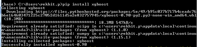
That’s all there is to it.

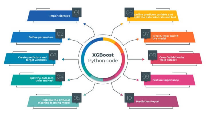
Awesome! Now we move to the real thing, ie the XGBoost python code.

We will divide the XGBoost python code into following sections for a better understanding of the model

Import libraries

We have written the use of the library in the comments. For example, since we use XGBoost python library, we will import the same and write # Import XGBoost as a comment.

Define parameters

We have defined the list of stock, start date and the end date which we will be working with in this blog.

Just to make things interesting, we will use the XGBoost python model on companies such as Apple, Amazon, Netflix, Nvidia and Microsoft. Creating predictors and target variables

We have also defined a list of predictors from which the model will pick the best predictors. Here, we have the percentage change and the standard deviation with different time periods as the predictor variables.

Create predictors and target variables

The target variable is the next day's return. If the next day’s return is positive we label it as 1 and if it is negative then we label it as -1. You can also try to create the target variables with three labels such as 1, 0 and -1 for long, no position and short.

Let’s see the code now.

Before we move on to the implementation of the XGBoost python model, let’s first plot the daily returns of Apple stored in the dictionary to see if everything is working fine.

Output:

Yes. It all looks fine!

Initialise the XGBoost machine learning model

We will initialise the classifier model. We will set two hyperparameters namely max_depth and n_estimators. These are set on the lower side to reduce overfitting.

Output:

XGBClassifier
XGBClassifier(base_score=None, booster=None, callbacks=None,
              colsample_bylevel=None, colsample_bynode=None,
              colsample_bytree=None, device=None, early_stopping_rounds=None,
              enable_categorical=False, eval_metric=None, feature_types=None,
              gamma=None, grow_policy=None, importance_type=None,
              interaction_constraints=None, learning_rate=None, max_bin=None,
              max_cat_threshold=None, max_cat_to_onehot=None,
              max_delta_step=None, max_depth=3, max_leaves=None,
              min_child_weight=None, missing=nan, monotone_constraints=None,
              multi_strategy=None, n_estimators=100, n_jobs=None,
              num_parallel_tree=None, random_state=42, ...)

Define predictor variable and split the data into train and test

Since XGBoost is after all a machine learning model, we will split the data set into test and train dataset.

Create, train and fit the model

We will train the XGBoost classifier using the fit method.

Output:

XGBClassifier
XGBClassifier(base_score=None, booster=None, callbacks=None,
              colsample_bylevel=None, colsample_bynode=None,
              colsample_bytree=None, device=None, early_stopping_rounds=None,
              enable_categorical=False, eval_metric=None, feature_types=None,
              gamma=None, grow_policy=None, importance_type=None,
              interaction_constraints=None, learning_rate=None, max_bin=None,
              max_cat_threshold=None, max_cat_to_onehot=None,
              max_delta_step=None, max_depth=3, max_leaves=None,
              min_child_weight=None, missing=nan, monotone_constraints=None,
              multi_strategy=None, n_estimators=100, n_jobs=None,
              num_parallel_tree=None, random_state=42, ...)

Cross Validation in Train dataset

All right, we will now perform cross-validation on the train set to check the accuracy.

Output:

Accuracy: 49.28% (1.55%)

The accuracy is half the mark. This can be further improved by hyperparameter tuning and grouping similar stocks together. I will leave the optimisation part on you. Feel free to post a comment if you have any queries.

Feature Importance

We have plotted the top 7 features and sorted them based on their importance.

Output:

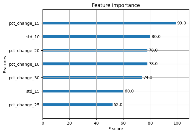
That’s interesting. The XGBoost python model tells us that the pct_change_15 is the most important feature out of the others. Since we had mentioned that we need only 7 features, we received this list. Here’s an interesting idea, why don’t you increase the number and see how the other features stack up, when it comes to their f-score.

You can also remove the unimportant features and then retrain the model. Would this increase the model accuracy?

We will leave that for you to verify.

Prediction Report

Output:

              precision    recall  f1-score   support

          -1       0.50      0.47      0.48       314
           1       0.50      0.53      0.51       315

    accuracy                           0.50       629
   macro avg       0.50      0.50      0.50       629
weighted avg       0.50      0.50      0.50       629

Hold on! We are almost there. Let’s see what XGBoost tells us right now:

That’s interesting. The f1-score for the long side is much more powerful compared to the short side. We can modify the model and make it a long-only strategy.

Let’s try another way to formulate how well XGBoost performed.

Confusion matrix

Output:

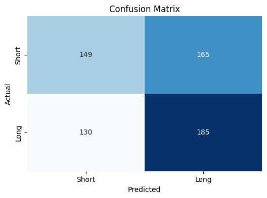
But what is this telling us?

Well it’s a simple matrix which shows us how many times XGBoost predicted “buy” or “sell” accurately or not.

For example, when it comes to predicting “Long”, XGBoost predicted it is right 185 times whereas it was incorrect 165 times.

Another interpretation is that XGBoost tended to predict “long” more times than “short”.

Individual stock performance

Let’s see how the XGBoost based strategy returns held up against the normal daily returns i.e. the buy and hold strategy. We will plot a comparison graph between the strategy returns and the daily returns for all the companies we had mentioned before.

The code is as follows:

Output:

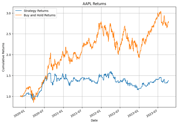
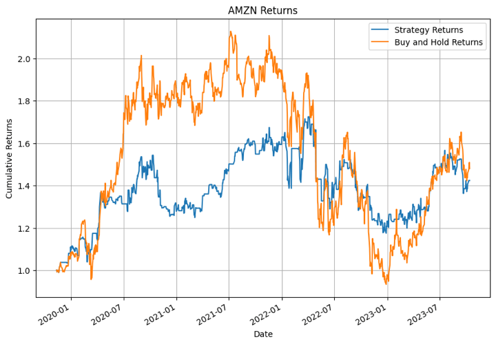
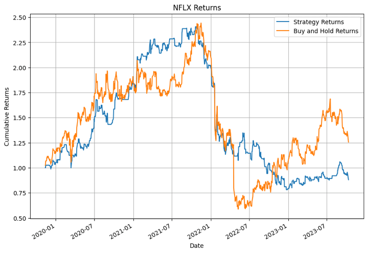
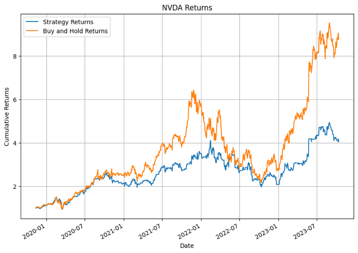
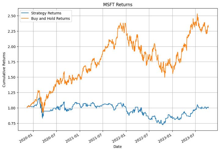
In the output above, the XGBoost model performed the best for NFLX in certain time periods. For other stocks the model didn’t perform that well.

Performance of portfolio

We were enjoying this so much that we just couldn’t stop at the individual level. Hence we thought what would happen if we invest in all the companies equally and act according to the XGBoost python model.

Let’s see what happens.

Output:

Date
2021-01-27    0.006411
2021-01-28   -0.011020
2021-01-29    0.021461
2021-02-01    0.011586
2021-02-02   -0.006199
dtype: float64

Now, we will calculate the cumulative returns of the portfolio.

Output:

Date
2021-01-27    1.006411
2021-01-28    0.995321
2021-01-29    1.016682
2021-02-01    1.028461
2021-02-02    1.022086
dtype: float64

Finally, let us visualise the cumulative returns of the portfolio.

Output:

Well, remember that these are cumulative returns, hence it should give you an idea about the performance of an XGBoost model with regard to the portfolio.

Pros of using XGBoost model in trading

XGBoost (Extreme Gradient Boosting) is a popular machine learning algorithm that has several advantages when applied to trading and financial prediction tasks.

Here are some of the pros of using XGBoost models in trading:

• High Predictive Accuracy: XGBoost is known for its high predictive accuracy. It can capture complex relationships in financial time series data, making it effective for forecasting price movements, volatility, and other market indicators.
• Handling Non-Linear Relationships: Financial markets often exhibit nonlinear behaviour. XGBoost can capture these non-linear relationships effectively, which is crucial for making accurate predictions in trading.
• Feature Importance Analysis: XGBoost provides feature importance scores, which can help traders and analysts understand which features (indicators) are driving the model's predictions. This can be valuable for decision-making and model interpretation.
• Ensemble Learning: XGBoost is an ensemble learning method, which combines the predictions of multiple weak models to create a strong model. This helps reduce overfitting and increase model generalisation.
• Regularisation Techniques: XGBoost supports L1 (Lasso) and L2 (Ridge) regularisation, which can improve the model's robustness and prevent overfitting, especially when dealing with high-dimensional financial data.
• Efficiency: XGBoost is optimised for speed and efficiency. It is parallelisable and can handle large datasets efficiently. This is important in trading, where timely decisions are critical.
• Outliers Handling: XGBoost can handle outliers in the data effectively. Outliers are common in financial data and can significantly impact the model's performance.
• Cross-Validation and Hyperparameter Tuning: XGBoost makes it easy to perform cross-validation and hyperparameter tuning, allowing traders and data scientists to fine-tune the model for better performance.
• Scalability: XGBoost can be used for both small- and large-scale trading operations. Its scalability makes it suitable for a wide range of trading strategies.
• Community and Resources: XGBoost has a large and active user community. This means that traders and developers have access to a wealth of resources, libraries, and online discussions for support and learning.
• Compatibility with Various Data Formats: XGBoost can work with different types of data, including numerical, categorical, and text data, making it versatile for various trading strategies.

In addition to the advantages mentioned above, one must be aware that domain expertise and careful feature engineering are essential for successful trading models.

You can learn feature engineering to combine it with XGBoost and help make the model more effective while trading.

Challenges of using XGBoost model in trading

Using the XGBoost model or any machine learning model in trading comes with several challenges, despite its potential benefits.

Here are some of the challenges associated with using the XGBoost model in trading:

• Data Quality and Preprocessing: High-quality, clean, and reliable data is crucial for training machine learning models. In the world of trading, data can be noisy, inconsistent, and subject to errors. Preprocessing the data, dealing with missing values, and ensuring data quality can be a significant challenge.
• Overfitting: XGBoost is prone to overfitting, especially when there are many features or the model is too complex. Overfitting occurs when the model fits the training data too closely, capturing noise and making it less effective at generalising to unseen data. Proper regularisation and feature selection are required to mitigate this issue.
• Feature Engineering: Designing effective features for trading data can be challenging. Domain-specific knowledge is essential for creating informative features that capture relevant patterns in financial data. The choice of features greatly influences model performance.
• Non-Stationarity: Financial markets are dynamic and non-stationary, meaning that the statistical properties of the data change over time. Models trained on historical data may struggle to adapt to changing market conditions, requiring constant retraining and monitoring.
• Evaluation and Backtesting: Evaluating the performance of trading models requires appropriate metrics and thorough backtesting. Selecting meaningful evaluation metrics and creating realistic backtesting environments is challenging and can impact model assessment.
• Model Interpretability: XGBoost is a powerful model but is often considered a "black box." Understanding the model's predictions and providing explanations for trading decisions can be difficult.
• Regulatory and Compliance Issues: Trading is subject to various regulatory and compliance requirements. Implementing machine learning models for trading must consider these constraints and ensure compliance with financial regulations.

Tips to overcome the challenges of XGBoost model

To overcome the challenges associated with using the XGBoost model in trading, several strategies and best practices can be applied.

• Firstly, it's crucial to start with high-quality data. This means obtaining data from reputable sources and conducting thorough data preprocessing. This may include data cleaning, standardisation, and handling missing data effectively through imputation or interpolation.
• Feature engineering is a key aspect of model development. By leveraging domain knowledge, you can create informative features that capture relevant patterns in financial data. These features can include technical indicators, sentiment analysis, macroeconomic variables, and market-specific data.
• Mitigating overfitting is another critical consideration. You can use proper regularisation techniques to prevent overfitting, such as adjusting hyperparameters like "max_depth" and "min_child_weight." Employing cross-validation helps assess model performance and ensures it generalises well to unseen data.
• Model hyperparameter tuning is essential for optimising model performance. Extensive tuning efforts using techniques like grid search or randomised search can help find the best hyperparameters, such as learning rate, number of estimators (trees), and subsample ratio.
• Regularly updating your trading model is necessary to adapt to changing market conditions. Using rolling windows of data for training allows the model to capture recent market dynamics and improves adaptability.
• Effective risk management should be integrated into your trading strategies. Robust risk management practices limit exposure to market risk. Diversifying trading strategies and assets spreads risk across different trading models and instruments.
• Model interpretability is essential. Techniques that help interpret model decisions and provide explanations for trading recommendations, such as SHAP (Shapley Additive exPlanations), can enhance trust and understanding of the model's behaviour.
• Regulatory compliance is a vital consideration. Ensure that your trading strategies and models comply with financial regulations and industry standards. Seek legal and compliance advice when necessary to navigate regulatory challenges.
• Creating a robust machine learning pipeline that automates data collection, preprocessing, feature engineering, model training, and deployment is essential. Continuous monitoring and maintenance are critical for model updates and adapting to data changes.
• Incorporate risk and portfolio management strategies into your approach to optimise asset allocation and position sizing. Diversifying portfolios and implementing strategies that are uncorrelated can help reduce overall risk.
• Continuous learning and staying up to date with advancements in machine learning and trading strategies are essential. Participation in relevant courses, seminars, and conferences can expand your knowledge.
• Collaboration with experts in data science, quantitative finance, and trading is essential. This can provide valuable insights and leverage collective expertise to address the challenges of using the XGBoost model effectively in trading.

Conclusion

We began our journey by delving into the fundamentals, starting with the inception of machine learning algorithms, and progressed to the next level, known as ensemble learning. We explored the concept of boosted trees and their invaluable role in enhancing predictive accuracy.

Ultimately, we arrived at the pinnacle of this learning journey, the XGBoost machine learning model, and uncovered its superiority over conventional boosted algorithms. Along the way, we delved into a straightforward Python code for XGBoost, using it to create a portfolio based on the trading signals it generated. Additionally, we examined feature importance and explored various parameters inherent to XGBoost.

If you're eager to embark on a structured learning path encompassing the entire lifecycle of developing machine learning trading strategies, you have the opportunity to enrol in our course on Natural Language Processing in Trading. With this course, you will learn to quantify the news headline and add an edge to your trading using the powerful model, that is, XGBoost.

Download Data File

• XGBoost with Python.ipynb

Login to Download

Author: Chainika Thakar (Originally written by Ishan Shah and compiled by Rekhit Pachanekar)

Note: The original post has been revamped on 4th December 2023 for accuracy, and recentness.

Disclaimer: All data and information provided in this article are for informational purposes only. QuantInsti^® makes no representations as to accuracy, completeness, currentness, suitability, or validity of any information in this article and will not be liable for any errors, omissions, or delays in this information or any losses, injuries, or damages arising from its display or use. All information is provided on an as-is basis.