Having its origin in 1964, CAPM or Capital Asset Pricing Model is an extremely relevant part of financial management and is an easy model to understand as well as apply. This model focuses on the sensitivity of the asset’s rate of return to the presence of a risk which befalls the entire stock market and is known as systematic risk.
It takes into account several assumptions and shows how the risk of investing in a particular asset defines the amount of return the investor will gain out of it. This relationship between risk and premium gained for bearing the risk is the core of CAPM. Yet, there are other concepts that surround the model which this article has covered.
Furthermore, in the same model, calculation of risk is essential for getting the right estimate of return or premium on that risk. Apart from this model, there are other models as well which we will discuss for Asset Pricing. In this article, we will go through:
- CAPM and its Working
- Uses and Assumptions of CAPM
- How do you calculate Beta and what is the Capital-Security Market Line?
- Two Primary Benefits and Two Limitations of the Model
- Other Factor Models of Asset Pricing
CAPM and its Working
Capital Asset Pricing Model is quite a useful one which helps you get a fair understanding of the relationship between the estimated return on an investment and its risk or systematic risk.
Now, systematic risk is that amount of risk which you may bear on a specific investment in the market. Some examples of such a diversified risk are wars, recession, etc. Whereas, this model assumes that there are particular kinds of financial assets which may be available with zero risk on returns.
In such a time, this model gives you the decisiveness for diversification of the assets in your portfolio. This diversification of the assets is useful in hedging against the risks of investment in particular financial assets.
Hence, the systematic risk on return is over and above the risk-free return on investment. And, this model tells you whether the investment is worth the risk or not.

In the visual above, it is clearly visible that you have two options, which are, to opt for:
- Risk-free Return on Investment which has no risk and 5% of estimated return on investment
or
- Systematic risk on Investment which has a higher amount of risk but also a higher amount of estimated return on the investment (compared to risk-free return), which is 10%.
To decide between the two options, CAPM Model comes in handy.
Let us now see the formula for CAPM which gives you an estimated return on investment for you to be able to decide which option is more profitable. And, the formula is:
R = Rf + 𝝱 * (Rm - Rf)
In the formula above,
Ra = Estimated return on the investment
Rf = The Risk-free rate of return on an investment
𝝱 = Beta value or risk value of investing in financial asset
Rm = Average return in the capital market
So, the formula above calculates Estimated return on the investment, which is aimed to give you an estimate of the rate of return you will get by investing in a risky asset. You will be able to find this estimate by applying the formula above.
In the formula, the risk of investing in that asset (𝝱) is multiplied with the Market Risk Premium i.e., (Rm - Rf) to get the amount over and above the Risk-free return which you will get if you invest in a risk-free financial asset.
And, adding the output with the Risk-free rate of return on investment in any other financial asset in the market will give you the Premium (total estimated return) you get rewarded with for bearing that risk.
Conclusively, this estimate is to help you get higher yields while you invest in high-risk financial assets.
For an instance,
Assume the following for asset XYZ:
Rf = 3%
Rm = 10%
𝝱 = 0.75
By using CAPM, the rate of return in asset XYZ:
Ra = 0.03 + [0.75 * (0.10 - 0.03)]
0.0825 = 8.25%
If an investor wants a return of 10% for his/her investment, then as per CAPM model, he/she should not invest in XYZ. But, if the investor seeks a return less than 8.25%, say 7%, then it is better to invest in XYZ.
Coming to the types, there are two types of risks that this model covers, and they are:
- Systematic Risk
- Unsystematic Risk
Both these risks were mentioned by financial economist William Sharpe, who created the Capital Assets Model. He began the model with the thought that any investment can have two types of risks.
Systematic Risk
This one implies the market risks which are always attached to investing and hit the entire stock market altogether. For instance, in case of recession, the investment in the stock market is bound to be riskier than other times. In such a time, this model helps you decide which stocks will be more profitable or less risky.
Unsystematic Risk
This type of risk is called the “specific risk” as it is related to the individual stocks. This risk does not relate to the general market’s move as a whole. Hence, this risk is related to a particular stock in the market which befalls an investor because of any of the business failures.
It is important to understand here that the Specific or Unsystematic Risk can be dealt with by optimizing the portfolio. This is a relevant observation mentioned in the Modern Portfolio theory.
However, in case of Systematic risk, optimization of the portfolio helps but comparatively lesser than it does in the Unsystematic Risk. As we mentioned above, the factors leading to Systematic risk bring the entire market under their ambit. Hence, it is the Systematic Risk which affects the investors most. And, that is how this model focuses on managing Systematic Risk.
Now, let us see the Assumptions and Uses of CAPM.
Uses and Assumptions of CAPM
Here, we will see the well-known Assumptions on which CAPM exists and also the Uses of the model in different fields.
Since the assumptions are important for any model, the Capital Asset Model also works on some assumptions mentioned by the economist William Sharpe who created this model:
- Diversified portfolios of investors
- Single-period transaction
- Risk-free rate of return
- Existence of perfect capital market
Diversified portfolios of investors
This implies that the investors will be needing the return only for the Systematic Risk in their portfolios as the Unsystematic Risk can be diversified with ease. Hence, Unsystematic Risk has been ignored in this model.
Single-period transaction
There is a standard holding period assumed in the model so as to make the returns on the different stocks comparable. Hence, a holding period of one year is used for all the stocks. This is done because a stock with a holding period of 5 months can not be compared with a stock of 12 months’ holding period.
Risk-free rate of return
This assumption states that the investors can borrow as well as lend at the risk-free rate of return. This assumption was made by the Modern Portfolio Theory from which this model was derived in the first place.
Existence of perfect capital market
According to this assumption, all the stocks are valued rightly and their rate of returns will be accurately estimated. A perfect capital market means that there are no taxes or costs; the perfect information is readily available to the investors and that there are a large number of traders in the market.
Okay Now! Let us move to the implementations/uses of CAPM.
Since Capital Asset Pricing Model provides an insight into pricing of stocks and determines the expected returns, it has its Implementations/Uses in:
- Investment Management
- Corporate Finance
Investment Management
CAPM is one model which has been an important tool for many investors, and particularly the portfolio managers. This is possible because CAPM provides the expected or estimated return on the investment by taking into consideration the Beta or risk value of investing in the stock. This estimation helps to understand which stocks to invest in and which not. Hence, this way the investors can invest in the High-Beta securities (where Beta is more than 1) in case the market is rising. Whereas, they can invest in Low-Beta securities (where Beta is less than 1) in case the market is expected to fall or is falling.
Its working in Investment Management is straightforward as we discussed in the first section "CAPM and its Working".
Corporate Finance
In Corporate Finance, this model holds a lot of importance since it suggests the cost of equity as the least expected return for the particular company’s stock. This cost of equity is nothing but the return that the firm or company pays to the shareholders for investing in their stock (riskier stock). This stock’s expected return is, in turn, the shareholder’s opportunity cost of investing in the equity funds of the company.
So, in simple words, Capital Asset Model helps the company or the firm employing the equity funds to get an estimated rate of return. On the basis of this estimation, the company offers the rate of return to the shareholders of the company. Now, since the company has got an estimation, it must earn at least the cost on the equity-based portion of its funds or the stock price is bound to fall in the market.
On the contrary, if the company finds it difficult to earn the cost of equity, it must not continue holding the shares or the funds of the shareholders. This is important because this way, the shareholders will be saved from bearing the opportunity cost. Further, the shareholders can invest in some other stocks in the financial market where they expect to earn the same expected return at the same level of risk. Now, an important observation here is that this cost of equity is difficult to find unless we use CAPM here.
Let us see how to use CAPM in calculating the cost of equity which is also called the Weighted Average Cost of Capital (WACC).
Cost of equity or WACC
Now, the formula for WACC or Cost of equity helps to determine as to how much exactly can you expect the flow of return in a specified amount of time. Let us see this with an example. Here, to help you understand how CAPM helps in calculating Cost of equity, we will take the same example of XYZ company as we did in the explanation of CAMP. The formula for Cost of equity is:
Cost of equity = Cash flow today/(1+ra)t
So, we have used the example of CAPM below.
Assume the following variables for your company XYZ:
ra = ?
rf = 3%
rm = 10%
βa = 0.75
By using CAPM, the rate of return in asset XYZ:
ra = 0.03 + [0.75 * (0.10 - 0.03)]
0.0825 = ra
Now, going forward, 8.25% is the expected return on the asset which is the percentage by which you can calculate and decide the Cost of equity. Let us assume that a cash flow in XYZ of $1000 is done. But, as the cash is more valued today, we will calculate its value in 2 years.
Cash invested today - $1000
Cost of equity (considering discounted value of cash) - $1000/(1+ra)t = $1000/(1+0.0825)t = $1000/(1+0.0825)2
= $853.9
Thus, $853.9 is the future value of your cash flow in the current time period. This gives you the estimate so that you decide your cost of equity below this calculation.
Let us now go ahead and see how to calculate Beta and what does the Capital-Security Market Line imply.
How do you calculate Beta and what is the Capital-Security Market Line?
As the Capital Asset Pricing Model suggests, Beta is one and only significant variable for measuring a stock’s risk. This is done by finding out the stock’s volatility in the market. This implies that the model compares the upward or downward movement of the particular stock with the upward or downward movement of the stock market as a whole.
So, if a stock’s price moves in the same manner as the market or somewhere around the whole stock market, then that stock’s Beta is taken as 1. A stock with the Beta value more than 1 will be considered a riskier stock and less than 1 will be considered a less risky stock. This implies that a more risky stock must provide the market risk premium or, in simple words, more return as compared to the less risky stock or the risk-free asset.
Hence, the Beta portrays that the investment which is riskier than the risk-free investment should be able to earn a premium (additional return) over the risk-free return on investment.
After understanding all about Beta being the amount of calculated risk of investing in a particular asset in the market, let us now see how to calculate Beta in Python.
Output:
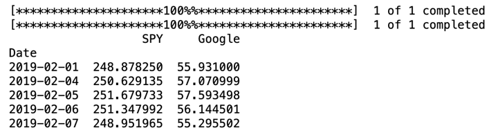
Running the code above gives the output with the prices of both the stocks in January and February.
Then, with the help of Linear Regression, we find the Beta of Google.
Output: 0.4149313287632459
Running the above code, gives us the Beta of Google stock which is 0.4149313287632459. Since 0.41 is lesser than the market average which is achieved when Beta is 1, we will consider this stock to be a less risky stock.
Perfect! After seeing how to calculate Beta in Python, we will move over to another important measure which is Capital-Security Market Line. In this concept, there are two Market Lines known as:
- Capital Market Line and
- Security Market Line
Capital Market Line (CML)
In the case of Capital Market Line, there is a representation of the relationship between standard deviation of market (risk) and the expected return of market portfolio.
In CML, we use:
- Standard deviation as risk and
- All the financial investments available to the proportion of the same in the market as the market portfolio.
Also, the slope of the Capital Market Line represents the price of Market risk here.
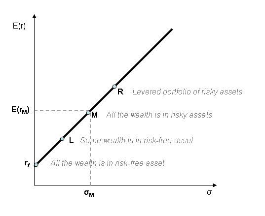
In the image above, you can see that the model takes Standard deviation as risk on the x-axis and Expected return of the market or the Market portfolio on the y-axis which includes the return on risk-free assets.
As you can see, this model shows:
rf = The entire investment or wealth in risk-free asset
L = Some or a percentage of investment or wealth in a risk-free asset while other in the asset having systematic risk (between rf and L).
M = Entire investment or wealth in assets bearing systematic risk.
R = Portfolio of all the risky assets.
Hence, the conclusive portfolio is the reward to the investor for bearing the risk of holding the portfolio for a particular amount of time.
Here, the formula of Expected return on market portfolio is:
E(RP) = Rf + σp((Rm - Rf) / σm)
In the formula:
E(RP) = Expected return of the market portfolio
Rf = Risk-free rate of return for investing
σp = Standard deviation of a portfolio
σm = Standard deviation of market
Rm = Rate of return of the market
Now, we will see the representation of the relationship between Risk-free asset and Portfolio SD or Portfolio Standard Deviation in Python. In the code below, we have imported matplotlib for plotting the graph. After that we have called the CML function for putting the formula for Portfolio SD and Portfolio return. Then, we go on giving the labels to x-axis and y-axis of the graph and finally, we plot the graph.
As we run the code above, we get the following output:
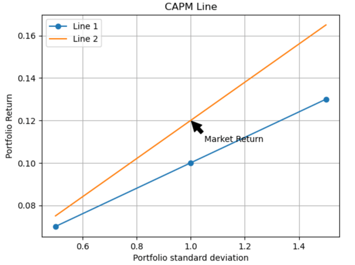
Hence, the CML or the Capital Market Line helps to find out the Expected return on the market portfolio of the investor.
Security Market Line (SML)
Security Market Line is a tool for evaluating the investment and has been derived from CAPM. This evaluation tool is devised for seeing the risk-return proportion for different securities. Also, the assumption of this tool is that the investor needs to be compensated for two things:
- Time Value of money
- Corresponding level of risk of investing in any asset.
Here also, Beta is taken into consideration like in CAPM. In the SML, the Beta of the security is taken as the Systematic risk and hence, as we mentioned above, this risk is for the entire market as a whole. Therefore, diversification of the portfolio will not be able to eliminate this risk.
In this tool, different Beta values show different amounts of risks in comparison with the market average. Let us see what each Beta value represents.
- Beta value 1 shows that the stock’s risk is the same as the overall average of the market.
- Beta value which is higher than 1 shows that the risk level for investing in the particular stock is more than the market average.
- Beta value which is lesser than 1 shows that the risk level is below the market average.
Now, let us see the formula for plotting Security Market Line, which is a simple one and it is:
Rr = Rf + β + (Rm - Rf)
In the formula,
Rr = Required return
Rf = Risk-free rate of return
β = Beta value or risk of investing in the security
Rm = Market return
(Rm - Rf) = Market risk premium
SML is usually used for comparison between two or more similar securities having an estimated rate of return which is the same. But, the important role here is of the Beta value which is the risk value.
In such a case, you will be needing SML to find out as to which security bears more risk in relation to the estimated or expected rate of return.
In another case, SML can be to find out as to which security offers more amount of rate of return between the one bearing equal risk.
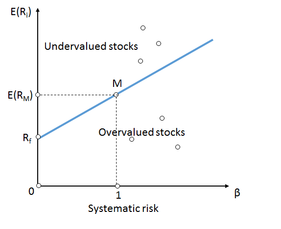
In the image above, we have a graphical representation of SML. Here, x-axis shows Beta value and y-axis shows Expected rate of return which includes Risk-free assets and Expected market return.
Now, 1 on x-axis shows the Beta value or risk of 1 which is the same as market average. Also, it shows the Market risk premium between Rm and R0 for the same amount of risk. Further, if the Beta value goes above 1, then the risk to invest in the particular security will increase and so will the Market risk premium.
In simple words, the investor will be compensated or rewarded further for investing in higher risky assets.
Above and below the SML, there are two observations:
- Assets which are above the SML are undervalued assets because they offer higher expected return for the given amount of risk.
- Assets which are below the SML are overvalued assets because they offer lesser expected returns for the same amount of risk.
Also, the slope will be as steep as the amount of market premium. Hence, higher the market premium, steeper the slope.
Hence, the CAPM describes the market behaviour, whereas, SML gives the expected return on the stock.
Now, let us move ahead and see the Primary Benefits and Limitations of CAPM.
Two Primary Benefits and Two Limitations of the Model
There are various benefits of the model, but we are seeing the two primary ones and also some of the limitations of the model. Let us first see the two primary benefits that this model holds which also explain its popularity.
- Firstly, this model takes into consideration the systematic risk which shows the real-world market or reality. This assumption also supports the frequent empirical research and testing and hence, is more close to real market scenario than other models.
- Secondly, this model is much better when it comes to calculating cost of equity as compared to the dividend growth model.
Now, let us see the limitations of the model which make the model unpopular amongst some others.
Firstly, it is not clear whether the model works or not. Since it assumes that an investor can earn more only by investing in the riskier stocks, its relevance is somewhat debatable. It was observed by economists like Kenneth French and Eugene Fama that the differences in Betas over a lengthy period of time does not really explain the performance of different stocks. Also, the linear relationship between Beta and stock return breaks down after a short period of time.
Secondly, to use the model, some values are needed to be assigned on the variables. There are some values like Equity risk premium which are difficult to find. Although, the Beta values are now calculated and also readily available on the internet for all the stock-exchange listed firms. The limitation is that the unpredictability may arise in the value of expected return since the value of Beta is not constant and continuously changes over a period of time.
Great! Now, we will see the other two models which can be used for Asset Pricing ahead.
Other Factor Models of Asset Pricing
It is interesting to know that the Capital Asset Pricing Model is not the only model for Asset Pricing and there are other models for the same. Here, we will see two such models which are:
- Three-Factor Model
- Five-Factor Model
Three-Factor Model
This is also known as the Fama and French model, and since it is called the Three-Factor Model, it is quite self-explanatory that it has three-factors which it depends on. Those three-factors are:
- Size of firms
- Book-to-book market values
- Excess return on the market.
The formula for the Three-Factor Model is:
R = Rf + 𝝱 * (Rm - Rf) + bs . SMB + bv . HML + 𝞪
Here,
R = Portfolio's expected rate of return
Rf = Risk-free rate of return
Rm = Return of the market portfolio
𝝱 = Analogous to classical 𝝱 but not equal to it
SMB = Small Minus Big market capitalization
HML = High Minus Low book-to-market ratio
Also, both SMB and HML measure the historic excess returns of small caps over big caps and of value stocks over growth stocks.
Five-Factor Model
The Fama-French five-factor model is yet to be proven as an improvement compared to previous models. It is known as Five-Factor Model, because it includes two more factors known as:
- Profitability and
- Investment
Most investors still use the famous three-factor model but as industry professionals have some doubts regarding their relevance, it has got neglected. Seeing the practical relevance of the work done by Fama and French, it surely seems that it would be in the best interest of investors if they use the Five-Factor model.
The formula for Five-Factor model is:
Rit - RFt = ai + bi (RMt - RFt ) + siSMBt + hIHMLt + riRMWt + ciCMAt + eit
Here,
Rit = The return in month t of one of the portfolios
RFt = Risk-free rate
RMt - RFt = The return spread between the capitalization weighted stock market and cash
siSMBt = The return spread of small minus large stocks (the size effect)
hIHMLt = The return spread of inexpensive minus expensive stocks (the value effect)
riRMWt = The return spread of the most profitable firms minus the least profitable
ciCMAt = The return spread of firms that invest conservatively minus aggressively (AQR,2014)
If you see above in the formula, ai + bi (RMt - RFt ) is nothing but the CAPM.
Great! Now, as we have reached the end of the article we will see what all we covered so far.
The following video that explains - “Portfolio Assets Allocation: A practical and scalable framework for Machine Learning Development” by Raimondo Marino from Milan, Italy and “Portfolio Optimization for Dividend Stocks” by Kurt Selleslagh from Singapore.
This Portfolio Assets Allocation with Machine Learning article is the final project submitted by the author Raimondo Marino as a part of his coursework in the Executive Programme in Algorithmic Trading (EPAT) at QuantInsti.
Conclusion
In this article, we have covered some of the most important aspects of the Capital Asset Pricing Model. This article aimed to cover some of the essential topics to get an overview of the model. Also, in the end we discussed two other models for Asset Pricing briefly, which are an improvement over the Capital Asset Pricing Model. Moreover, it will be fair to mention that this is not it, since there is still space for some more models ahead for providing improved versions.
Download Data File
- CAPM.ipynb
Disclaimer: All data and information provided in this article are for informational purposes only. QuantInsti® makes no representations as to accuracy, completeness, currentness, suitability, or validity of any information in this article and will not be liable for any errors, omissions, or delays in this information or any losses, injuries, or damages arising from its display or use. All information is provided on an as-is basis.