By Rushda Ansari and Palak Khanna
Performance and risk metrics are widely used to evaluate the performance of a stock or portfolio, and forms a major component of portfolio management. In this blog, we will try to touch upon some important portfolio and risk metrics that can provide you with a clear view of your investment’s performance and risk.
The first part of the article looks at such commonly used performance metrics that give us an insight into the anatomy of a trading strategy. In the second part of the article, we will cover some important metrics for risk management in an investment or a portfolio. The final part explains strategy optimisation for your portfolio in brief with a simple example.
- Why do we need portfolio risk management?
- What are performance and risk metrics?
- Types of performance metrics and their calculation
- Types of risk metrics and their calculations
- How to measure trading performance of a portfolio?
- What is strategy optimisation?
- An example of strategy optimisation
Why do we need portfolio risk management?
The performance of a portfolio of assets is measured with a set of parameters.
For example, if you are trading in equity then your returns are compared against the benchmark index. The consistency of returns of the portfolio also proves to be a significant factor.
But returns alone cannot measure the success or failure of a portfolio. In finance, risk and return are considered to be two sides of the same coin. You can’t have one without the other.
Therefore, identifying and analysing the risk undertaken in your investment is a crucial step while evaluating and optimising your trading strategy.
When asked what the stock market will do, Benjamin Graham said, “It will fluctuate”.
There is no sweeping method by which one can predict the exact movement of the market direction. Hence, it is important that we make use of multiple risk and performance metrics while making investment decisions.
What are performance and risk metrics?
A key lesson for portfolio risk management is that returns mean nothing unless we put them side by side with the risk undertaken. Performance and risk metrics do just that.
Performance and risk metrics are statistics we use to analyse our trading strategy. They can help determine:
- how well your trading strategy performs,
- how robust it is, and
- if it will survive in different market conditions.
We use these metrics to get a better understanding of an investment's return by measuring how much risk is involved in producing that return.
Let's now look at some useful performance and risk management trading measures to help you evaluate your investment portfolio.
Types of performance metrics
The various types of performance metrics are as follows:
Absolute risk-adjusted measures
Sharpe ratio
Sharpe Ratio measures the average return earned in excess of the risk-free rate per unit of volatility or total risk i.e., standard deviation.
In other words, the ratio describes how much profit you receive for the extra volatility you endure for holding a riskier asset. Sharpe ratio is one of the most popular metrics among investors to measure portfolio performance.
Remember, you need compensation for the additional risk you take by not holding a risk-free asset.
Formula and calculation for Sharpe ratio
$$ Sharpe ~Ratio=\frac{R_p-R_f}{\sigma_p} \\ $$Where,
\(R_p\) = Return of the portfolio
\(R_f\) = Risk-free rate
\(σ_p\) = Standard deviation of the portfolio’s excess return
Sharpe ratios greater than 1 are preferable, as it means your returns are greater given the risk you are taking. So generally, the higher the ratio, the better the risk to return scenario for your portfolio.
Sortino ratio
Sortino ratio is a modified version of the Sharpe ratio that differentiates harmful volatility from the overall volatility. It is calculated by estimating the excess portfolio return over the risk-free return relative to its downside deviation (i.e. standard deviation of negative asset return).
In addition to focusing only on portfolio returns that fall below the mean, the Sortino ratio is thought to offer a better representation of risk-adjusted performance since positive volatility is a benefit. Like Sharpe ratio, a higher value of Sortino ratio indicates less risk relative to return.
Formula and calculation for Sortino ratio
$$ Sortino ~Ratio=\frac{R_p-R_f}{\sigma_d} $$Where,
\(R_p\) = Actual or expected return of the portfolio
\(R_f\) = Risk-free rate
\(σ_d\) = Standard deviation of the downside
Calmar ratio
Calmar Ratio also called the Drawdown ratio is calculated as the Average Annual rate of return computed for the latest 3 years divided by the maximum drawdown in the last 36 months.
The higher the ratio, the better is the risk-adjusted performance of an investment fund such as hedge funds or commodity trading advisors (CTAs) in the given time frame of 3 years.
Formula and calculation for Calmar ratio
$$ Calmar ~Ratio=\frac{R_p-R_f}{Maximum Drawdown} $$Where,
\(R_p\) = Return of the portfolio
\(R_f\) = Risk-free rate
\(R_p - R_f\) = Annual rate of return
The annual rate of return shows how a fund has performed over a year. The maximum drawdown is characterised as a maximum loss from peak to trough over a given investment period.
It is determined by subtracting the fund’s lowest value from its highest value and then dividing the result by the fund’s peak value.
Relative return measures
Up capture ratio
The Up capture ratio measures a portfolio’s return with respect to the benchmark’s return.
It is used to analyse the performance of a portfolio during bull runs, i.e. when the benchmark has risen. A ratio greater than 100 indicates that the portfolio has outperformed the index.
Formula for Up capture ratio
The up capture ratio is calculated by dividing the portfolio’s returns by the returns of the index during the bullish trend and multiplying that factor by 100.
$$ Up ~capture ~ratio = \frac{Portfolio ~returns ~during ~bull ~runs}{Benchmark ~returns}~*100 $$Down capture ratio
A statistical measure that measures the portfolio’s return with respect to the benchmark’s return.
The downside capture ratio is used to analyse how a portfolio performed during a bearish trend, i.e. when the benchmark has fallen. A ratio less than 100 indicates that the fund has outperformed the index.
Formula for Down capture ratio
The down capture ratio is calculated by dividing the portfolio’s returns by the returns of the index during the bearish trend and multiplying that factor by 100.
$$ Down ~capture ~ratio = \frac{Portfolio ~returns ~during ~bear ~runs}{Benchmark ~returns}~*100 $$Up percentage ratio
The Up percentage ratio compares the number of periods a portfolio outperformed the benchmark when the benchmark was up. The higher the ratio the better is the performance of the portfolio.
Formula for Up percentage ratio
$$ {\small Up ~percentage ~ratio = \frac{No. ~of ~periods ~portfolio ~outperformed ~benchmark ~in ~bull ~runs}{No. ~of ~periods ~the ~benchmark ~was ~up}~*100} $$Down percentage ratio
The Down percentage ratio is a measure of the number of periods that a portfolio outperformed the benchmark when the benchmark was down.
This is then divided by the number of periods that the benchmark was down. The higher the ratio the better is the performance of the portfolio.
Formula for Down percentage ratio
$$ {\small Up ~percentage ~ratio = \frac{No. ~of ~periods ~portfolio ~outperformed ~benchmark ~in ~bear ~runs}{No. ~of ~periods ~the ~benchmark ~was ~down}~*100} $$Types of risk metrics
The types of risk metrics are divided into:
Absolute risk measures
Variance
Variance expresses how much the rate of return deviates from the expected return i.e. it indicates the volatility of an asset and hence is considered as a risk indicator.
Therefore, it can be used by the portfolio manager to assess the behaviour of the assets under consideration. A large variance indicates greater volatility in the rate of return.
Formula and calculation for Variance
Variance is calculated as the average of the squared deviations from the mean. To compute variance all you need to do is calculate the difference between each point within the dataset and their mean. Then, square the differences and average the results.
$$ \sigma^2 = \frac{\sum_{i=1}^n(x_i-x_{mean})^2}{n-1} $$Where,
\(x_i\) = the ith data point
\(x_{mean}\) = the mean of all data points
n = the number of data points
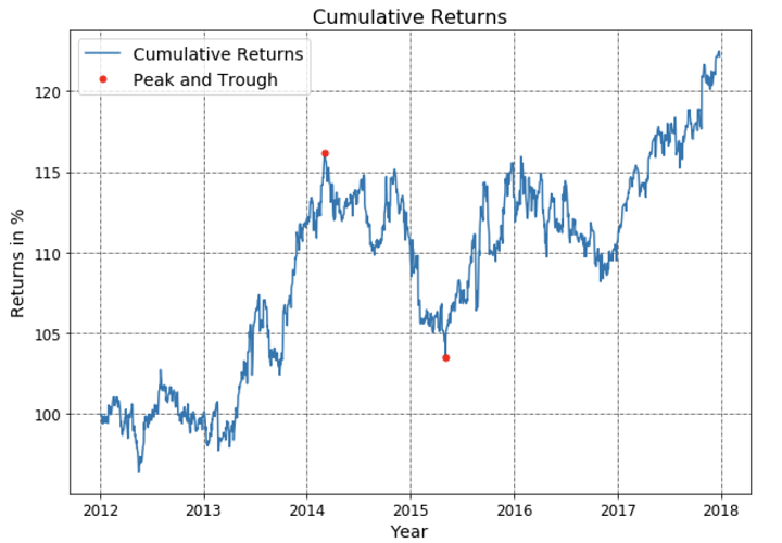
Maximum Drawdown
Maximum Drawdown is one of the key measures to assess the risk in a portfolio. It indicates the downside risk of a portfolio over a specified time period.
It signifies the maximum loss from a peak to a trough of a portfolio’s equity and is expressed in percentage terms.
A lower maximum drawdown implies slight fluctuations in the value of the investment and, therefore, a lesser degree of financial risk, and vice versa.
Below you can see a plot of a portfolio’s cumulative returns. Its maximum drawdown, from peak to trough, is represented by the red points as shown.
Formula and calculation for Maximum Drawdown
Maximum drawdown is given by the difference between the value of the lowest trough and the highest peak before the trough.
It is generally calculated over a long period of time when the value of an asset or an investment has gone through several boom-bust cycles. The formula for calculating Maximum Drawdown is shown below:
$$ Maximum ~Drawdown = \frac{Trough ~value- Peak ~value}{Peak ~value} $$Relative risk measures
Correlation Coefficient
The concept of correlation is really to see if two variables are similar to each other or opposite to each other. The correlation coefficient tells you how strongly any two variables, say x and y, are related.
It takes values only between -1 and 1. A correlation of -1 means that as x increases, y will decrease. Hence they will move exactly opposite to each other. While a correlation equal to 1 means that as x increases y will also increase.
A correlation of 0 means that x and y have no linear relationship in their movement. The correlation between two variables is particularly helpful when investing in the financial markets.
For example, correlation can help you in determining how well a stock performs relative to its benchmark index, or another fund or asset class. Also, By adding low or negatively correlated assets to your existing portfolio, you can gain diversification benefits.
Formula and calculation for Correlation Coefficient
To calculate the correlation coefficient, we must first determine the covariance of the two variables. Next, you should calculate each variable's standard deviation, which is nothing but the square root of the variance.
Now we can find the correlation coefficient. It is determined by dividing the covariance with the product of the two variables' standard deviations. Now, let's look at the formula for covariance and correlation.
$$ Cov(x,y) = \frac{\sum(x_i-x_m)(y_i-y_m)}{n-1} \\ \rho_{xy}=\frac{Cov(x,y)}{\sigma_x\sigma_y} $$Where,
\(⍴_xy\) = correlation coefficient
\(x_i, y_i\) = data values of x and y for i= 1,2…n
\(x_m, y_m\) = the means of x and y, respectively
\(σ_x, σ_y\) = standard deviations of x and y, respectively
\(n\) = the number of data points
Beta
Beta measures the volatility of a stock or a portfolio in relation to the market. Beta for the market is always equal to one.
So, if a portfolio has beta greater than 1, it is considered to be more volatile than the market; while a beta less than 1 means less volatility. Beta values are not bounded like the correlation values.
Formula and calculation for Beta
To calculate the beta of an asset or portfolio, we must know the covariance between the return of the portfolio and the returns of the market. We will also need the variance of the market returns.
$$ Beta = \frac{Cov(r_i,r_m)}{Var(r_m)} $$Where,
\(r_i\) = expected returns from your portfolio
\(r_m\) = expected returns from the market
Tail risk measures
Value-at-Risk (VaR)
Value at Risk (VaR) is a statistical measurement used to assess the level of risk associated with a portfolio. The VaR calculation measures the maximum potential loss with a degree of confidence for a specified period.
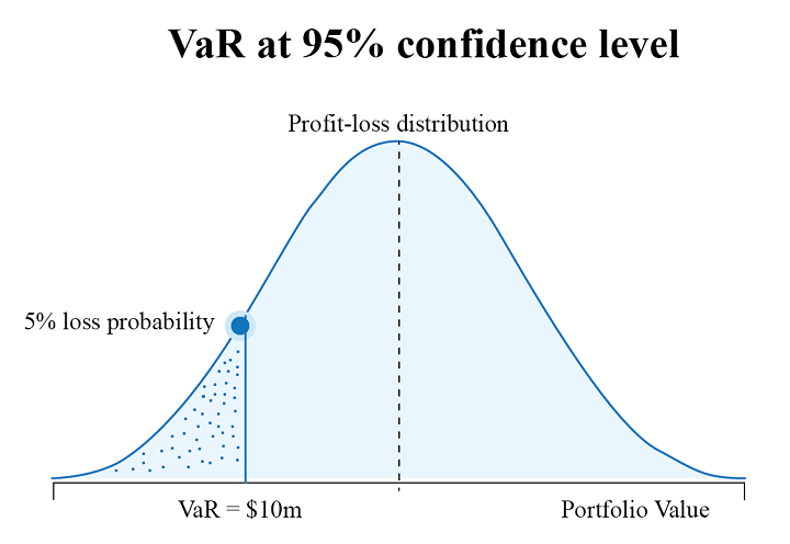
For example, as illustrated above, if the VaR for a portfolio is at 10 million at 95% confidence level, then it means that in 5% of cases the loss will exceed the VaR amount.
However, you should note that VaR does not say anything about the size of the losses within this 5%.
Formula and calculation for VaR
There are mainly three methods to calculate VaR. These are the historical method, the variance-covariance method, and the Monte Carlo simulation method. Value at Risk (VaR) calculations can also be carried out using Excel or Python.
Conditional Value-at-Risk (CVaR)
Conditional Value-at-Risk, also known as Expected Shortfall (ES), is a risk assessment measure that quantifies the amount of tail risk in an investment portfolio. It is computed by taking a weighted average between the VaR value and the losses exceeding VaR.
As you can see below, CVaR is seen as an extension of VaR and is considered superior to VaR as it accounts for losses exceeding VaR. Therefore, you can use CVaR in your portfolio optimisation strategy to get a better idea of extreme losses and effectively manage your portfolio risk.

How to measure trading performance of a portfolio?
What is the first thing that you look at to gauge the performance of a portfolio? If your answer is high returns, then like most investors, you too think that high returns translate to the excellent performance of a portfolio, but this is only partly true.
While returns do contribute to performance measurement, it is also important to assess the risk undertaken to achieve these returns. Contrary to popular beliefs, the portfolio with the highest returns is not the most ideal portfolio.
To determine the performance of the portfolio, it is necessary to measure the risk-adjusted returns. We have already discussed the various absolute risk-adjusted measures of performance above.
However, it’s also necessary that you understand the various aspects of portfolio analysis, ie. performance measurement and evaluation.
What is strategy optimisation?
Let’s say you have developed a strategy and measured its performance and risk metrics.
How will you know if this strategy garners the best results?
And if there is a scope for improvement, wouldn’t you want to make your strategy perform better?
That’s exactly why the process of strategy optimisation is carried out.
So, you:
- develop a strategy,
- measure its performance,
- optimise it, and
- rebuild on the basis of optimisation.
The optimisation allows a strategist to improve the results of their strategy by fine-tuning the parameters and the formulae that drive the strategy. It can be done by fine-tuning a single parameter or a set of parameters to achieve the desired objective.
An example of a strategy optimisation objective can be maximising the total profits generated. Another objective of optimisation can be minimising the drawdowns.
Having mentioned the purpose of optimisation, one should also be aware that optimisation is like a double-edged sword.
If multiple rules are applied to training data during optimisation to achieve the desired equity curve, it results in over-fitting of the data and the model is likely to lose its forecasting ability on the test and future data.
The portfolio optimisation module is an important component of strategy development platforms. However, one should note that different platforms can offer different strategy optimisation tools and techniques.
Hence, one should evaluate the optimisation tools available before subscribing to any strategy development platform.
An example of strategy optimisation
Let us take an example of a simple strategy and use the “Riskfolio-Lib” library to optimise the strategy performance.
Riskfolio-Lib is a Python library specifically designed for portfolio optimisation and allocation. It focuses on four main objectives of optimisation, which include, maximising return, minimising risk, and maximising portfolio utility.
Let’s understand the steps to perform optimisation based on the objective of maximising risk-adjusted returns.
Step 1: Install the library
The very first step is to install the library. And to do so, you need to run the following code:
Step 2: Get the data
Let’s say we want to optimise a portfolio comprising four stocks: Microsoft, JP Morgan, Comcast, and Target. In that case, we need to first get the price data of these four stocks and then calculate their daily returns. You can do this by running the following lines of code:
Step 3: Create a portfolio and set the method for estimation
The next step is to create a portfolio and set the method to estimate the required parameters. In this case, it’s expected returns and covariance. We will be carrying out the estimation based on historical data. The following lines of code will help you do this:
Step 4: Optimise the portfolio
Now that we have everything that we need, we can finally optimise the portfolio with this single line of code:
The model is set to Classic because it’ based on historical data. Alternatively, you can set it to Black Litterman (BL) or Factor Model (FM). The risk measure (rm), in this case, is mean-variance (MV), and the object is Sharpe. We have used historical scenarios for risk measures that depend on scenarios, hence hist is set to “True”.
Output:
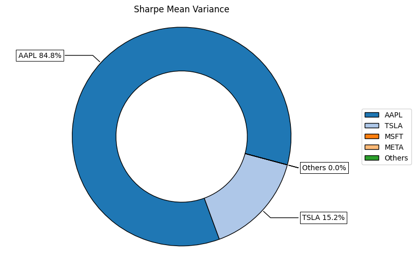
     Weights(%)
AAPL	84.77
TSLA	15.23
META	0.00
MSFT	0.00
Step 4: Plot the results
This step is optional. If you wish to visualise the results you can plot them using the same library.
To do so, you need to run the following lines of code:
Output:
Conclusion
Performance metrics are not only used to measure the performance of a portfolio but also to optimise it. In this blog, we have given you an overview of some commonly used portfolio metrics, risk metrics, and also covered the strategy optimisation concept with an example using the “Riskfolio-Lib” library.
A detailed study like this blog on portfolio optimisation methods compares the performance of an equally-weighted asset portfolio with the performance of an optimised portfolio.
To learn more about building a portfolio quantitatively, strategy optimization, and different portfolio management techniques such as Factor Investing, Risk Parity, Kelly Portfolio, and Modern Portfolio Theory, check out the course on Quantitative Portfolio Management by Quantra. It is a great way to learn how to construct a portfolio that generates returns and manages risks effectively using risk management metrics.
File in the download:
- Complete Python code - Example of Strategy Optimisation
Note: The original post has been revamped on 1st June 2022 for accuracy, and recentness.
Disclaimer: All investments and trading in the stock market involve risk. Any decision to place trades in the financial markets, including trading in stock or options or other financial instruments is a personal decision that should only be made after thorough research, including a personal risk and financial assessment and the engagement of professional assistance to the extent you believe necessary. The trading strategies or related information mentioned in this article is for informational purposes only.