Checkout our Latest Video that demonstrates how to build, simulate, and optimise a portfolio using Python and CVXPY. The session begins with foundational concepts of portfolio management, including asset allocation, expected return estimation, and risk modelling. It then transitions into hands-on coding, where Mohak constructs the efficient frontier by simulating thousands of random portfolio weights.
Download the codes here:
When constructing a multi-asset portfolio, coming up with the strategy to allocate weights to the portfolio components is a very important step in the process. Coming up with weights for a portfolio given its components can be done in a number of ways and is a question that boggles even the most skilled managers. So what is the most optimal way to do this? in this article we will try to introduce the most widely used methods and understand the intuition behind them.
When we think naively about this, the most intuitive way of allocating to the securities would be based on our conviction for them. In the early days of the financial market’s history traders actually used to do that and be profitable. As the trend following strategies saw crashes in early 1997 with increased volatility in the markets, traders started adding stop losses and take profits and staggered entry and exit to the strategies.
After the Global Financial Crisis in 2008 “risk-parity” became a widely followed strategy. This strategy allocated equal risk budgets to all participating assets and does not look at investor views or expected return projections. The most popular method that does incorporate views is the Markovitz Mean-Variance Optimal portfolio based on the Capital Asset Pricing Model or CAPM. The passive portfolios like the market index use a market-cap-weighted allocation. Other naive methodologies are the equal weight portfolio or the minimum variance portfolio.
The literature around portfolio optimization is rich and vast. There are a wide variety of variations and improvements upon the basic methods and a lot of active research that goes around it. I worked on a variation of risk parity called "risk budgeting" and a novel “active risk budgeting” when working on the US managed futures strategies. There is even a use case of machine learning methods like reinforcement learning methods that find a good fit for this problem.
In this post, we take an introductory glance at the rationale of some popular portfolio construction methods and their implementation in Python. We will also look at how each of these methods performs for an example portfolio consisting of sectoral indices published on the NSE namely, Bank, Auto, Fin Service, FMCG, IT, Media, Metal, Pharma, PSU Bank, Private Bank, Realty.
We rebalance our portfolios quarterly and trade in a long-only fashion.
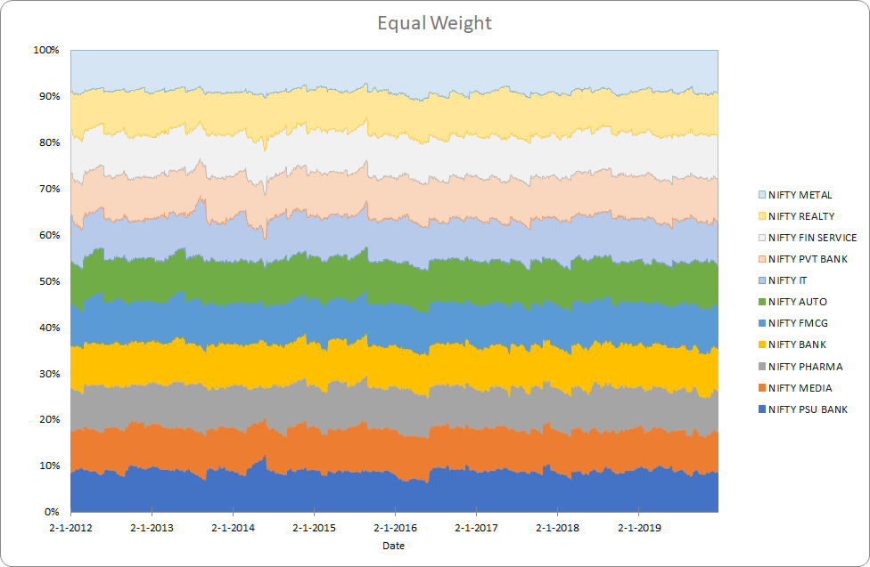
Equal Weight
This method assigns equal weights to all components. This would be most useful when the returns across all interested assets are purely random and we have no views.
def equal_weighted_portfolio(w, V):
''
The equal-weighted portfolio returns equal weights to each of the
portfolio components
'''
return [1.0/len(w)]*len(w)
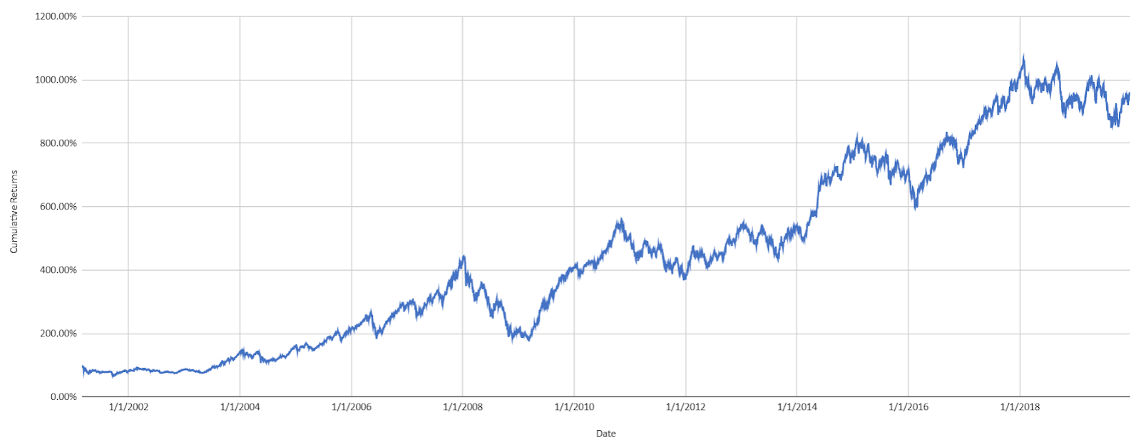
We’ll see the returns of an equal-weighted portfolio comprising of the sectoral indices below.

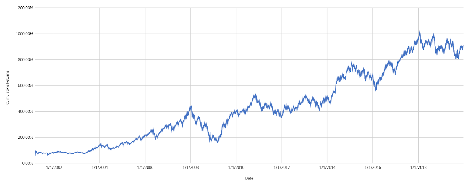

The annualized return is 13.3% and the annualized risk is 21.7%
Risk Parity
The risk contribution of each asset is equal. This method gained popularity after the 2008 crisis. Risk parity works best in a world where the Sharpe ratios between all asset classes are the same (and consequently equal risk contribution would contribute equal returns).
The weights are a solution to the optimization equation -
![]()
Where, w is the weight, ∑ is the covariance matrix and n is the number of assets
def risk_parity(w, V):
def calculate_portfolio_variance(w,V):
# function that calculates portfolio risk
w = np.matrix(w)
return (w*V*w.T)[0,0]
def calculate_risk_contribution(w,V):
# function that calculates asset contribution to total risk
w = np.matrix(w)
sigma = np.sqrt(calculate_portfolio_variance(w,V))
# Marginal Risk Contribution
MRC = V*w.T
# Risk Contribution
RC = np.multiply(MRC,w.T)/sigma
return RC

def risk_budget_objective(x,pars):
# calculate portfolio risk
V = pars[0]# covariance table
x_t = pars[1] # risk target in percent of portfolio risk
sig_p = np.sqrt(calculate_portfolio_variance(x,V))# portfolio sigma
risk_target = np.asmatrix(np.multiply(sig_p,x_t))
asset_RC = calculate_risk_contribution(x,V)
J = sum(np.square(asset_RC-risk_target.T))[0,0] # sum of squared error
return J

def total_weight_constraint(x):
return np.sum(x)-1.0
w0 = x_t = [1.0/len(w)]*len(w)
cons = ({'type': 'eq', 'fun': total_weight_constraint})
res= minimize(risk_budget_objective, w0, args=[V,x_t], method='SLSQP',constraints=cons, options={'disp': True})
return np.asmatrix(res.x)

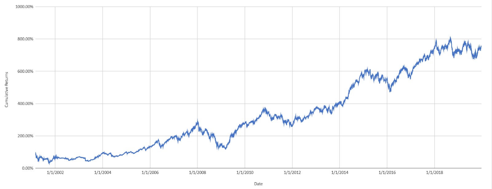
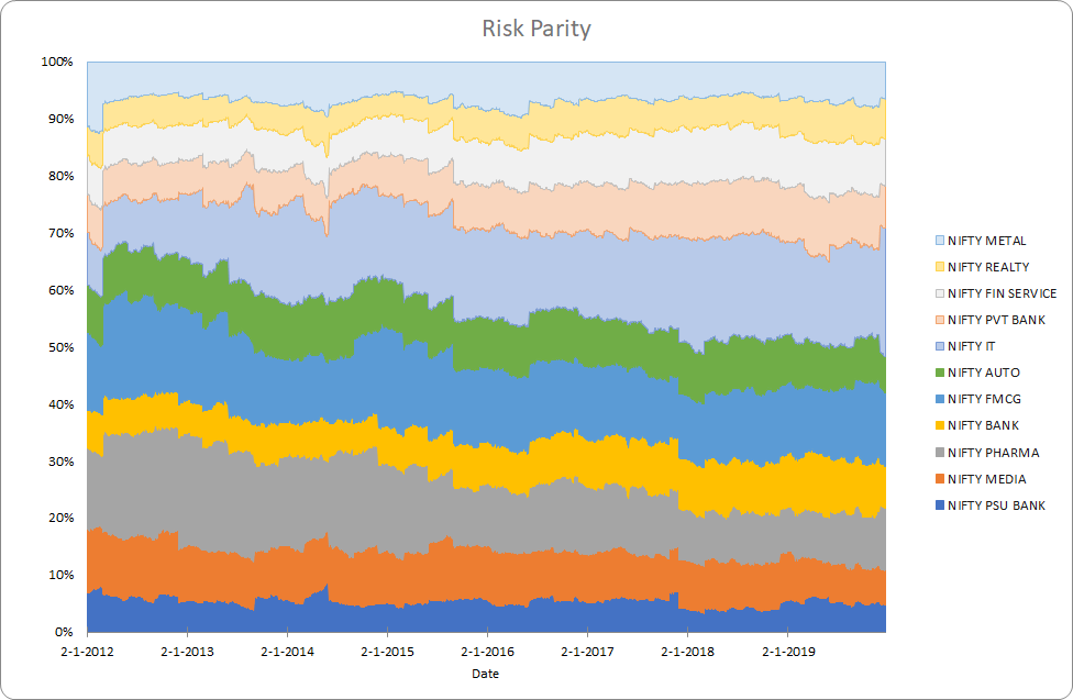
The annualized return is 13.40% and the annualized risk is 24.7%. We can see that low volatility sector like FMCG get higher weight and high-risk sectors like PSU Bank get lower weight.
Minimum Variance
This method minimizes the portfolio’s volatility. This would work best when the returns are not proportional to risk and lowering risk does not lead to lower returns as well.
The weights are a solution to the equation,
![]()
Where, w is the weight, ∑ is the covariance matrix
def minimum_variance(w0, V):
def calculate_portfolio_var(w, pars):
# function that calculates portfolio risk
V = pars # covariance table
w = np.matrix(w)
return (w * V * w.T)[0, 0]
def total_weight_constraint(x):
return np.sum(x) - 1.0
cons = ({'type': 'eq', 'fun': total_weight_constraint})
res = minimize
calculate_portfolio_var,
w0,
args=V,
method='SLSQP',
constraints=cons,
options={
'disp': False})
return np.asmatrix(res.x)

The annualized return is 13.6% and the annualized risk is 20.8%. This looks quite similar to the equal weight example and could be because the risks of the indices are similar and the optimizer based solution to low-risk portfolio stops at a local minimum.
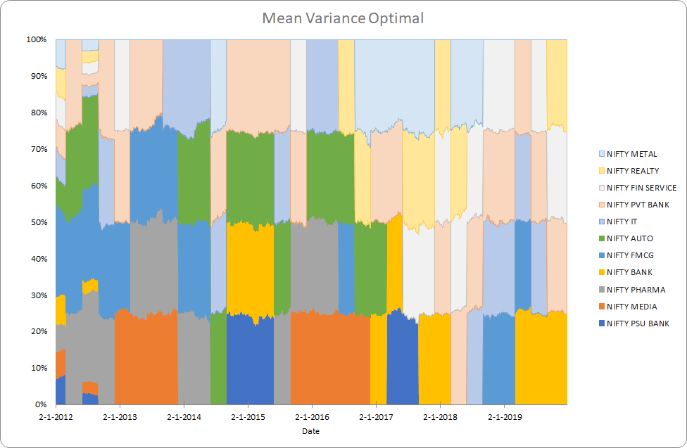
Mean-Variance Optimization
This is the famous Markovitz Portfolio. This is a mathematical framework for assembling a portfolio of assets such that the expected return is maximized for a given level of risk.
The weights are a solution to the optimization problem for different levels of expected returns,

![]()
Where, w is the weight, ∑ is the covariance matrix and N is the number of assets, R is the expected return and q is a "risk tolerance" factor, where 0 results in the portfolio with minimal risk and ∞ results in the portfolio infinitely far out on the frontier with both expected return and risk unbounded.
def mean_variance_optimization(w, V):
def calculate_portfolio_risk(w, V):
# function that calculates portfolio risk
w = np.matrix(w)
return np.sqrt((w * V * w.T)[0, 0])
def calculate_portfolio_return(w, r):
# function that calculates portfolio return
return np.sum(w*r)
# optimizer
def optimize(w, V, target_return=0.1):
init_guess = np.ones(len(symbols)) * (1.0 / len(symbols))
weights = minimize(get_portfolio_risk, init_guess,
args=(normalized_prices,), method='SLSQP',
options={'disp': False},
constraints=({'type': 'eq', 'fun': lambda inputs: 1.0 - np.sum(inputs)},
{'type': 'eq', 'args': (normalized_prices,),
'fun': lambda inputs, normalized_prices:
target_return - get_portfolio_return(weights=inputs,
normalized_prices=normalized_prices)}))
return weights.x
optimal_risk_all = np.array([])
optimal_return_all = np.array([])
for target_return in np.arange(0.005, .0402, .0005):
opt_w = optimize(prices=prices, symbols=symbols, target_return=target_return)
optimal_risk_all = np.append(optimal_risk_all, get_portfolio_risk(opt_w, V))
optimal_return_all = np.append(optimal_return_all, get_portfolio_return(opt_w, w))
return optimal_return_all, optimal_risk_all
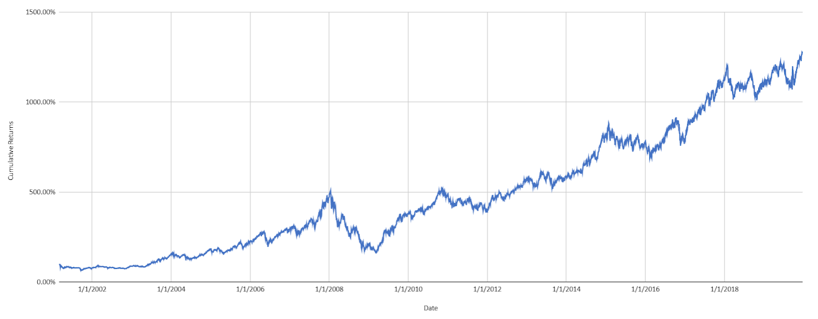
The annualized return is 15.2% and the annualized risk is 21.9%. We have taken the portfolio with the highest level of risk, one could actually choose a risk-based on her risk tolerance.
On an overall level, we see that mean-variance optimization is possibly the best method for our example.
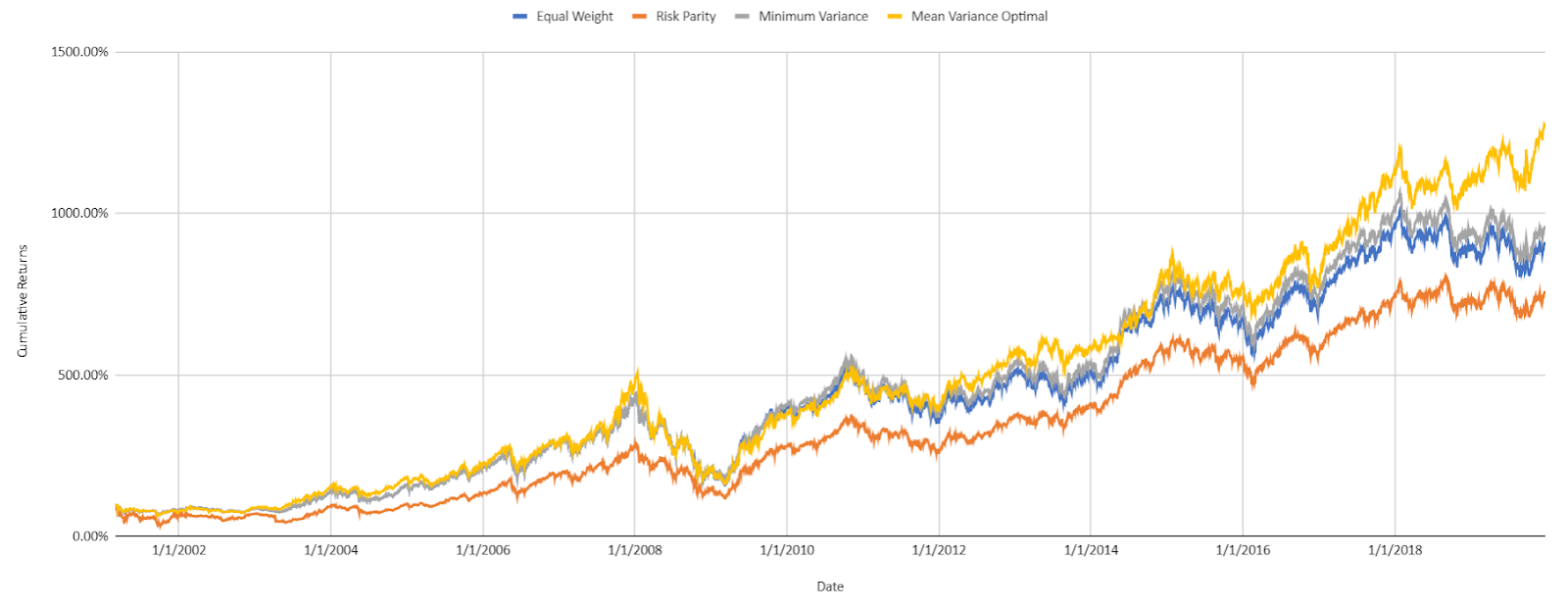
Now surely each of these methods could be of choice under different conditions contingent on different factors. So what are the factors to look at?
Factors Affecting Portfolio Optimization
Behavioural Factors
The investor's risk outlook or risk aversion is obviously the most important factor to keep in mind while deciding the portfolio construction method. The choice of instruments and the investment horizon guide the diversification available and the methodology so this is the most important factor.
Correlation
Correlation guides diversification. In their research posted recently Resolve Asset Management demonstrate that the optimization-based methods outperform naive methods only when there is an opportunity to diversify and a large number of risk factors present. For imperfectly correlated assets the portfolio returns and volatility are different from the weighted sum. So correlation plays a big role in the choice of the portfolio construction method.
Market Regime
We showed that minimum variance is optimal when all return assumptions are same and risk parity is optimal when all risk-adjusted returns are the same. Such scenarios actually occur as the markets change regimes. There are actual regimes where returns are inversely correlated to risk while others where higher risk is rewarded by higher returns. This makes market regimes a good factor to look at when evaluating the portfolio construction methods.
Conclusion
I hope this article gives the reader a good start in the exploration of the wonderful field of research on portfolio construction and optimization. This interesting area of research can add levels of sophistication to any systematic trading strategy, as covered in the options trading course.
Disclaimer: The views, opinions, and information provided within this guest post are those of the author alone and do not represent those of QuantInsti®. The accuracy, completeness, and validity of any statements made or the links shared within this article are not guaranteed. We accept no liability for any errors, omissions or representations. Any liability with regards to infringement of intellectual property rights remains with them.