Originally written by Apoorva Singh and Rekhit Pachanekar, Edited by Chainika Thakar
Welcome to a comprehensive guide on the Sharpe Ratio – a pivotal financial metric developed by Nobel laureate William F. Sharpe in 1966. This guide is designed for those seeking a deep understanding of how the Sharpe Ratio is calculated, interpreted, and applied for making informed investment decisions.
In finance, achieving high returns is a common goal, but understanding the associated risk is equally important. The Sharpe Ratio provides a quantitative measure of an investment's performance relative to its risk, offering a valuable tool for comparing and evaluating various investment opportunities.
Through this guide, readers will cover the basics of the Sharpe Ratio, its formula, practical calculations, and applications using real-world examples. We explore its role in portfolio comparison, performance evaluation, risk management, and benchmarking, making it a must-read for both novice investors and seasoned professionals.
Whether you aim to enhance your investment strategy, enrol in an algorithmic trading course, or grasp the foundations of risk-adjusted returns, this guide empowers you with the knowledge and skills needed to navigate the complexities of financial decision-making. Join us in unravelling the intricacies of the Sharpe Ratio and take a significant step towards optimising your investment journey.
This blog covers:
- What is Sharpe ratio?
- Formula of Sharpe ratio
- How to calculate Sharpe ratio?
- Example of Sharpe ratio
- Comparing Sharpe ratio with other performance metrics
- How to calculate Sharpe ratio in Excel?
- How to calculate Sharpe ratio in Python?
- Common misconceptions about Sharpe ratio
- Limitations of Sharpe ratio
- How to improve Sharpe ratio for your strategy?
- FAQs about Sharpe ratio
What is Sharpe ratio?
The Sharpe Ratio is a measure used to calculate the risk-adjusted return of an investment or a trading strategy. Developed by William F. Sharpe, a Nobel laureate, in 1966, it helps investors understand the return on investment compared to its risk.
The Sharpe ratio is widely utilised in portfolio risk management to evaluate the risk-adjusted performance of investment portfolios. Hence, Sharpe ratio plays an important role in portfolio analysis.
Here's how it's applied:
- Portfolio Comparison: Investors can use the Sharpe ratio to compare the risk-adjusted returns of different portfolios. A higher Sharpe ratio indicates better risk-adjusted returns, suggesting that the portfolio is generating more return per unit of risk taken.
- Performance Evaluation: Portfolio managers can assess the historical risk-adjusted performance of their portfolios over specific periods. By examining the Sharpe ratio over time, managers can gauge the consistency and efficiency of their investment strategies.
- Risk Management: The Sharpe ratio helps in understanding the trade-off between risk and return. Portfolio managers can adjust portfolio allocations to achieve a desired level of risk-adjusted return based on the insights derived from the Sharpe ratio.
- Benchmarking: The Sharpe ratio can be used as a benchmark to evaluate the performance of a portfolio against a relevant market index or peer group. This comparison aids in identifying whether the portfolio is outperforming or underperforming relative to its risk profile. The Sharpe Ratio is one of the most universally used performance benchmarks in quantitative trading, helping practitioners evaluate strategies objectively regardless of market conditions.
Formula of Sharpe ratio
Mathematically, the Sharpe Ratio is calculated as:
$$Sharpe \;Ratio = \frac{(Return\; of\; the\; portfolio\; or\; investment\;−\;Risk\; free\; rate)}{Standard\; deviation\; of\; the\; portfolio\; or\; investment}$$
Here's a breakdown of its components:
- Return of the portfolio or investment: The average return generated by the investment over a specific period.
- Risk-free rate: The return on an investment that is considered to have no risk, typically based on government bonds like U.S. Treasury Bills.
- Standard deviation: A statistical measure of the volatility or risk associated with the investment, representing how much the returns deviate from the average return.
How to calculate Sharpe ratio?
Once you see the formula, you will understand that we deduct the risk-free rate of return, which helps us figure out if the strategy makes sense.
If the Numerator turned out negative, wouldn’t it be better to invest in a government bond that guarantees you a risk-free rate of return?
Some of you would recognise this as the risk-adjusted return.
In the denominator, we have the standard deviation of the investment’s return. It
helps us identify the volatility and the risk associated with the investment. Thus, the Sharpe ratio helps us identify which strategy gives better returns compared to the volatility.
Also, a higher Sharpe ratio indicates a better risk-adjusted return, suggesting that the investment or strategy has generated more return for each unit of risk taken. Conversely, a lower Sharpe ratio suggests that the investment might not be adequately compensating the investor for the risk undertaken.
There, that is all when it comes to Sharpe ratio calculation.
Example of Sharpe ratio
Let’s take an example now to see how the Sharpe ratio calculation helps us.
You have devised a strategy and created a portfolio of different stocks. After backtesting, you observe that this portfolio, let’s call it Portfolio A, will give a return of 11%. However, you are concerned with the volatility at 8%.
Now, you change certain parameters and pick different financial instruments to create another portfolio, Portfolio B. This portfolio gives an expected return of 8%, but the volatility now drops to 4%.
Considering the fact that the risk-free rate of return is 3%, the Sharpe Ratio calculation for both portfolios is as follows:
|
Portfolio A |
Portfolio B |
|
|
Rate of return |
11 |
8 |
|
Risk-free rate of return |
3 |
3 |
|
Volatility |
8 |
4 |
|
Sharpe Ratio |
(11-3)/8 = 1 |
(8-3)/4 = 1.25 |
Thus, according to the Sharpe Ratio calculation, we should consider Portfolio B because even though the expected return is less than portfolio B, the volatility of portfolio B is less than portfolio A and thus, is less risky.
Currently, most exchange-traded funds provide the Sharpe ratio for their investments on their websites as well.
Sharpe Ratio can be used in many different contexts such as performance measurement, risk management and to test market efficiency. When it comes to strategy performance measurement, as an industry standard, the Sharpe ratio is usually quoted as “Annualised Sharpe”.
Annualised Sharpe is calculated based on the trading period for which the returns are measured.
If there are N trading periods in a year, the annualised Sharpe is calculated as:
$$Sharpe\;Ratio = \sqrt{N}\frac{E(R_x-R_f)}{StdDev(x)}$$
Here,
- N: Represents the number of periods (usually, it's the number of trading days or months). The square root of N is used to annualize the ratio. If you are calculating the Sharpe Ratio using daily returns, N would be the number of trading days in a year (typically 252), and if using monthly returns, N would be 12.
- E(Rx - Rf): This is the expected excess return of the investment or strategy, where Rx is the expected return of the investment, and Rf is the risk-free rate. The excess return is the return above and beyond the risk-free rate, compensating for the risk taken.
- StdDev(x): This is the standard deviation of the investment's returns. It measures the volatility or risk of the investment. The standard deviation indicates how much the values deviate from the mean (average).
Trade Level Sharpe ratio for Intraday Strategies
For an intraday trading strategy, instead of using the conventional Sharpe calculation, we can calculate the trade level Sharpe to get a better view of the strategy’s performance.
In this case, the risk-free rate can be considered to be 0 since there is no charge on interest. Sharpe ratio can be calculated by following these simple steps:
Imagine you have a trading strategy where you execute a series of trades, and for each trade, you record the profit and loss (PnL).
Here's a general example:
- Trade 1: +0.002 (Profit)
- Trade 2: -0.005 (Loss)
- Trade 3: +0.003 (Profit)
- Trade 4: +0.004 (Profit)
- Trade 5: -0.002 (Loss)
- Trade 6: +0.001 (Profit)
- Trade 7: -0.005 (Loss)
- Trade 8: +0.002 (Profit)
- Trade 9: -0.004 (Loss)
- Trade 10: +0.006 (Profit)
For these 10 trades, you can calculate the Sharpe Ratio using the formula:
$$Sharpe\;Ratio = \sqrt{N} \frac{mean(PnL)}{std\;dev(PnL)}$$- Mean of PnL: (0.002 - 0.005 + 0.003 + 0.004 - 0.002 + 0.001 - 0.005 + 0.002 - 0.004 + 0.006) / 10
- Standard Deviation of PnL: Calculate the standard deviation of the PnL values.
Let's say the mean is 0.001 and the standard deviation is 0.004. The Sharpe Ratio would then be:
Sharpe Ratio = 10 × (0.001/0.004)
Sharpe Ratio ≈ 10 × 0.25
Sharpe Ratio ≈ 0.25 × 3.162
Sharpe Ratio ≈ 0.7905
This gives you a measure of the risk-adjusted returns for your trading strategy. The higher the Sharpe Ratio, the better the risk-adjusted performance of the strategy.
Here's a simplified Python code example to demonstrate the calculation:
Output:
Mean of PnL: 0.0002
Standard Deviation of PnL: 0.003938414796731181
Sharpe Ratio: 0.16058631827165679
For high-frequency strategies, a large number of small successful trades for specific amounts smoothen the PnL curve and the standard deviation approaches zero which significantly spikes the Sharpe ratio, such that it might range in double digits.
On its own, any strategy with “annualised Sharpe ratio” of less than 1 (after including execution costs) is usually ignored. Most Quantitative hedge funds ignore strategies with an annualised Sharpe ratio of less than 2.
- For a retail algorithmic trader, an annualised Sharpe ratio greater than 1 is pretty good.
- For high-frequency trading, as discussed, the ratio can go up by double digits as well, especially for opportunity-driven but not highly scalable strategies.
The ratio is used by an individual when they are adding a new financial instrument to an existing portfolio, and they want to check how it impacts the portfolio.
Comparing Sharpe ratio with other performance metrics
Let us now compare the Sharpe ratio with other performance metrics below.
|
Metric |
Calculation Formula |
Focuses On |
Strengths |
Limitations |
|
Sharpe Ratio |
(Return of the portfolio or investment - Risk-free rate) / Standard deviation of the portfolio or investment |
Both upside and downside volatility |
Comprehensive measure of risk-adjusted returns; Suitable for all investments |
Sensitive to extreme values or fluctuations in the returns |
|
Sortino Ratio |
(Return of the portfolio or investment - Risk-free rate) / Downside standard deviation |
Only downside volatility |
Focuses on harmful volatility; More suitable for risk-averse investors |
Ignores upside volatility. Can be biassed towards strategies with more downside risk |
|
Treynor Ratio |
(Return of the portfolio or investment - Risk-free rate) / Beta |
Systematic (market-related) risk |
Evaluates returns relative to market risk; Suitable for diversified portfolios |
Ignores unsystematic (firm-specific) risk. Assumes market portfolio is efficient |
|
Jensen's Alpha |
Portfolio Return - (Risk-free Rate + (Market Return - Risk-free Rate)) |
Excess return over expected return |
Measures actual returns vs. expected returns given the portfolio's risk; Useful for active management |
Requires a benchmark index; Ignores other forms of risk |
|
Information Ratio |
(Portfolio Return - Benchmark Return) / Tracking Error |
Active return relative to a benchmark |
Measures the consistency of outperformance over a benchmark |
Relies on the accuracy of benchmark comparisons; Benchmark selection is crucial |
|
Calmar Ratio |
Compound Annual Return / Maximum Drawdown |
Risk-adjusted return relative to drawdown |
Emphasises return relative to the maximum loss; Suitable for trend-following strategies |
Sensitive to the time horizon; May not capture short-term volatility |
|
CAPM |
Expected Return = Risk-free Rate + Beta * (Market Return - Risk-free Rate) |
Systematic (market-related) risk and expected return |
Quantifies the relationship between expected return and systematic risk |
Assumes a linear relationship between risk and return; Ignores other sources of risk |
How to calculate Sharpe ratio in Excel?
Here are the steps to calculate the Sharpe Ratio in Excel using the formula:
Assuming:
- Rp is the annualised return on the investment.
- Rf is the risk-free rate.
- σ (sigma) is the standard deviation of the investment's returns.
Step 1: Collect Data
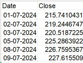
First of all, you need to download the data online. You can use yahoo finance or any data provider. I have taken the daily close price from 1 July 2024 to 31 December 2024 in this example.
You can arrange the data in the Excel sheet as shown below. This is a screenshot of the first few columns of the dataset.
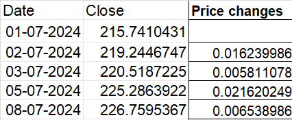
Step 2: Calculate the price change for daily returns
This is what the column for daily price change will look like. You simply need to apply the formula =((B3-B2)/B2) and then drag it down to other cells in the column “Price changes”.
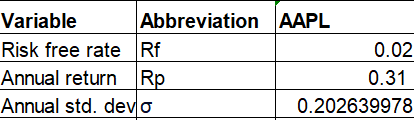
Step 3: Calculate the variables “Risk free rate (Rf)”, “Annual return (Rp)”, “Annual standard deviation ()”
This is how you can arrange the table for each variable required for calculating Sharpe ratio with the formula:
*Sharpe ratio = Rp - Rf / σ
This is how you will calculate each variable:
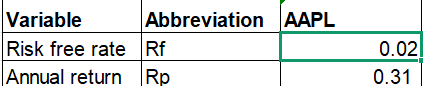
- Risk free rate (Rf): Rf will be assumed as 2% in this case. This is for illustration purposes only.
2. Annual return (Rp): First we calculate the mean daily returns as follows:
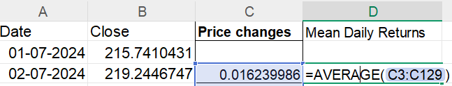
Then we annualise the mean daily returns by multiplying by 252, which is the approximate number of trading days in a year.
The calculation of Rp will require the formula as shown below.

The annual return is 0.31.
3. Annual standard deviation (): This will be calculated as shown below.
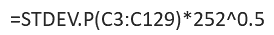
In the formula,
- C3 is the first price change
- C129 is the last price change
- 252 are the number of trading days in a year
- 252^0.5 is the square root of 252
Hence, by applying the formula, we get 0.2 as the calculated annual standard deviation.
Step 4: Calculate the Sharpe ratio
Now, we will calculate the Sharpe ratio as shown below.
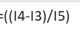
In the formula,
- I4 is the Annual return (Rp)
- I3 is the Risk free rate (Rf)
- I5 is the Annual standard deviation ()
In the image, (taken from Excel sheet) we can see that the calculated Sharpe ratio is 1.44.
Above you can see what the entire table with all the calculations looks like.
How to calculate Sharpe ratio in Python?
Going further, if you would like to find the Sharpe ratio on your own with Python code, below is how we can do it.
Let us see step by step process of the same.
Step 1: Import necessary libraries
Step 2: Fetch AAPL Stock data from Yahoo Finance for the period 2022-2024
Step 3: Calculate Short-term (50-day) and long-term (200-day) moving averages
Step 4: Generate Signals based on moving average crossover
Step 5: Calculate daily returns based on Signals
Step 6: Calculate cumulative returns
Step 7: Print the cumulative returns
Output:
Cumulative Strategy Return:
1.0439783521327737
Step 8: Plotting the Strategy Signals
Output:
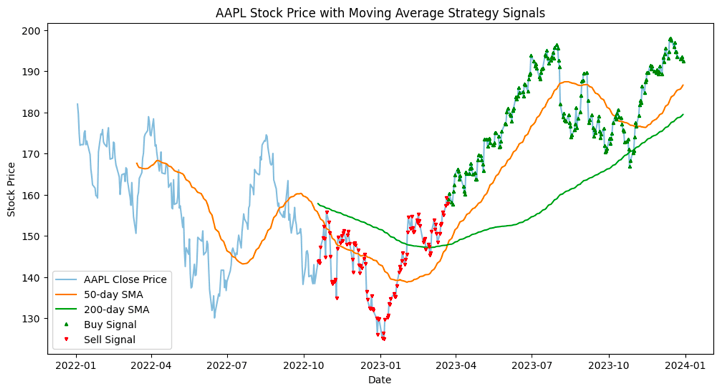
The plotted figure shows the historical stock price of AAPL along with two moving averages (50-day and 200-day) and signals generated by a simple moving average crossover strategy.
Let us see the breakdown of the plot’s components below.
AAPL Close Price Line:
The light blue line represents the daily closing prices of AAPL over the specified period.
50-day Simple Moving Average (SMA) Line:
The orange line represents the 50-day SMA of AAPL's closing prices. This line smoothens out short-term fluctuations and provides a trend-following signal.
200-day Simple Moving Average (SMA) Line:
The green line represents the 200-day SMA of AAPL's closing prices. This line smoothens out long-term fluctuations and provides a longer-term trend-following signal.
Buy Signals (Green Triangle '^'):
Green triangles indicate the points where the 50-day SMA crosses above the 200-day SMA, generating a buy signal. This crossover is considered bullish in technical analysis.
Sell Signals (Red Inverted Triangle 'v'):
Red inverted triangles indicate the points where the 50-day SMA crosses below the 200-day SMA, generating a sell signal. This crossover is considered bearish in technical analysis.
By observing the signals and moving averages, traders can potentially make decisions on when to enter or exit positions based on the strategy.
Step 9: Calculate Sharpe Ratio
Output:
Sharpe Ratio for the Strategy: 0.2954069610097365
Sharpe Ratio of 0.295 indicates a positive risk-adjusted performance for the investment or portfolio relative to a risk-free rate, suggesting that the investment has provided returns that justify the risk taken.
In the above code, we have assumed the risk-free rate of return as 5%, which can be changed accordingly.
**Note: The specific value for the risk-free rate used in the Sharpe Ratio calculation depends on the time frame and the currency in which the returns are measured. Commonly, the yield on short-term government securities, such as 3-month Treasury bills, is utilised.**
Common misconceptions about Sharpe ratio
The Sharpe Ratio is a widely recognized metric for evaluating the risk-adjusted performance of investments. However, several misconceptions surround its interpretation and application.
Here are some common misconceptions about the Sharpe Ratio:
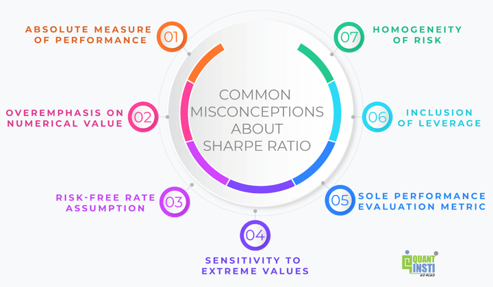
- Absolute Measure of Performance: One common misconception is viewing the Sharpe Ratio as an absolute measure of performance. While a higher Sharpe Ratio generally indicates better risk-adjusted returns, it's essential to compare it with relevant benchmarks or peer groups to assess relative performance accurately.
- Overemphasis on Numerical Value: Some investors may place excessive emphasis on achieving a specific Sharpe Ratio target without considering the underlying investment strategy, market conditions, or qualitative factors. The context in which the Sharpe Ratio is calculated is crucial for its meaningful interpretation.
- Risk-Free Rate Assumption: Another misconception is assuming a constant or universal risk-free rate for calculating the Sharpe Ratio across different markets or time periods. The choice of the risk-free rate should be appropriate and reflective of the investment's currency and duration.
- Sensitivity to Extreme Values: The Sharpe Ratio is sensitive to extreme values or outliers in return data. Some investors may misinterpret a sharp fluctuation in the Sharpe Ratio due to extreme returns as a significant change in risk-adjusted performance, while it might be a temporary anomaly caused by outliers.
- Sole Performance Evaluation Metric: While the Sharpe Ratio is a valuable metric, relying solely on it for evaluating investment performance can be limiting. Incorporating other performance metrics, qualitative analysis, and considering the broader investment context provides a more comprehensive assessment.
- Inclusion of Leverage: When comparing Sharpe Ratios across investments, it's essential to consider whether leverage or borrowed funds are used. A higher Sharpe Ratio resulting from leverage may not necessarily indicate superior investment skill but rather increased risk-taking.
- Homogeneity of Risk: Assuming that all investments have a similar risk profile or that the Sharpe Ratio provides a complete representation of an investment's risk characteristics is a misconception. The Sharpe Ratio focuses on volatility as measured by standard deviation but may not capture all aspects of an investment's risk, such as liquidity risk or geopolitical risk.
Limitations of Sharpe ratio in trading
The Sharpe Ratio is a widely used measure for assessing the risk-adjusted performance of an investment or portfolio. However, like any financial metric, it has its limitations.
Here is a table summarising some of the key limitations of the Sharpe Ratio:
|
Limitation |
Description |
|
Sensitivity to Return Distribution |
The Sharpe Ratio assumes that returns are normally distributed, but financial markets often exhibit non-normality, with fat tails and skewness. In the presence of extreme events or outliers, the Sharpe Ratio may not accurately reflect the risk associated with the investment. |
|
Dependency on Historical Data |
The Sharpe Ratio is based on historical data, and past performance does not guarantee future results. Changes in market conditions, economic factors, or the investment landscape may lead to different risk-return profiles in the future. Investors should be cautious when relying solely on historical Sharpe Ratios for decision-making. |
|
Single Metric for Portfolio Comparison |
When comparing multiple portfolios or investment strategies, the Sharpe Ratio may not provide a complete picture. It focuses on risk-adjusted returns but does not consider other important factors such as market exposure, style, or qualitative aspects of the investment process. Investors should use additional metrics and analysis for a comprehensive evaluation of investment options. |
|
Sensitivity to Benchmark Choice |
The choice of a benchmark index for comparison can significantly impact the Sharpe Ratio. Different benchmarks may lead to different risk-adjusted performance assessments. Investors should carefully select benchmarks that are relevant to the investment strategy and objectives. |
|
Time Period Dependency |
The Sharpe Ratio can vary depending on the chosen time period. Short-term fluctuations or market anomalies may have a more pronounced effect on the ratio in shorter time frames. Longer-term perspectives may provide a more stable assessment but could miss recent changes in risk-return dynamics. Investors should consider multiple time frames and analyse performance consistency. |
|
Ignores Non-Financial Considerations |
The Sharpe Ratio focuses exclusively on risk and return metrics, neglecting non-financial factors such as ethical considerations, social impact, and governance. Investors with specific non-financial criteria may need to complement the Sharpe Ratio with other metrics that address these aspects. |
|
Assumes Constant Risk-Free Rate |
The Sharpe Ratio assumes a constant risk-free rate over time. In reality, the risk-free rate can fluctuate, especially in response to economic conditions and central bank policies. Changes in the risk-free rate can impact the interpretation of the Sharpe Ratio, particularly when comparing performance across different time periods or economic environments. |
|
May Favour Strategies with Positive Skewness |
The Sharpe Ratio penalises strategies with negative skewness, which may not be suitable for all investors. Some investors may tolerate or even prefer downside protection over upside potential. The Sharpe Ratio does not differentiate between upside and downside volatility, and strategies with positive skewness (favourable asymmetry) may receive higher Sharpe Ratios even if they do not align with an investor's risk preferences. |
How to improve Sharpe ratio for your strategy?
Here are some tips which can help improve your strategy’s Sharpe ratio.
Risk Management
- Implement a robust strategy to limit potential losses.
- Consider stop-loss orders, position sizing based on volatility, or diversification.
Transaction Costs
- Factor in transaction costs and slippage in your strategy.
- Optimise trade execution to minimise costs.
Optimise Parameters
Fine-tune strategy parameters (e.g., moving average lengths) for maximum risk-adjusted returns.
Include Transaction Costs in Backtesting
Ensure that backtesting accounts for realistic transaction costs to reflect real-world trading conditions.
FAQs about Sharpe ratio
Here are some of the most frequently asked questions about Sharpe Ratio:
Q. What are the best practices for Sharpe ratio calculation?
A: Here you can see some of the best practices as per the experience of some professional traders:
- Consistent Time Period: Ensure that the return data and risk-free rate are consistent and aligned for the chosen time period.
- Accurate Risk-Free Rate: Use an appropriate risk-free rate that matches the investment's currency and duration.
- Robust Data Handling: Handle outliers or extreme values in return data appropriately to avoid distortion in the Sharpe Ratio calculation.
- Benchmark Comparison: Consider comparing the calculated Sharpe Ratio with relevant benchmarks or peer groups for context and relative performance assessment.
Q. What is meant by Sharpe ratio in modern portfolio theory?
A: The Sharpe Ratio plays a crucial role in Modern Portfolio Theory (MPT) by helping investors construct efficient portfolios that maximise returns for a given level of risk. MPT emphasises diversification and the benefits of combining assets with different risk-return profiles to achieve optimal portfolio allocation.
Q. What is the impact of Sharpe ratio on investment strategy?
A: The Sharpe Ratio influences investment strategy by guiding decisions on asset allocation, risk management, and performance evaluation. A thorough understanding of the Sharpe Ratio helps investors optimise their portfolios, aligning investments with their risk tolerance and return objectives, and ultimately enhancing long-term investment outcomes.
Q: What is a good Sharpe ratio?
A: Good Sharpe ratio indicates superior risk-adjusted returns, generally above 1. For example, 1.5 means your excess return over the risk-free rate is 1.5 times your portfolio's volatility.
Q: What is a high Sharpe ratio?
A: High Sharpe ratio signifies exceptional performance, typically exceeding 2. This suggests your portfolio generates significantly higher returns compared to its risk level.
Q: What is a negative Sharpe ratio?
A: Negative Sharpe ratio means your portfolio suffers losses exceeding the risk-free rate. This implies your chosen investments are underperforming even compared to a safe option like government bonds.
Q: What is a conditional Sharpe ratio?
A: The conditional Sharpe ratio measures risk-adjusted returns under specific market conditions, like rising or falling interest rates. It helps assess how your portfolio performs in different scenarios.
Conclusion
The Sharpe Ratio, a pivotal metric in finance, measures an investment's risk-adjusted return, aiding in portfolio evaluation, risk management, and strategy formulation. Developed by William F. Sharpe compares an asset's excess return to its volatility, with higher values indicating superior risk-adjusted performance.
However, misconceptions and limitations exist, necessitating a nuanced approach. By integrating the Sharpe Ratio with other metrics and best practices, investors can optimise portfolio performance, aligning with Modern Portfolio Theory principles and enhancing investment strategies for long-term success.
Ready to elevate your trading strategy? Enroll now in our course on Backtesting Trading Strategies and gain the essential skills to validate, refine, and optimise your trading rules. Unlock the power of historical data analysis, apply risk management measures, and avoid common backtesting pitfalls. Make informed decisions, minimise errors, and increase your trading success. Don't miss out – secure your spot today and take the first step towards mastering backtesting for trading excellence!
Files in the download
- Sharpe ratio calculation in Python
Note: The original post has been revamped on 13th February, 2024 for accuracy, and recentness.
Disclaimer: All investments and trading in the stock market involve risk. Any decision to place trades in the financial markets, including trading in stock or options or other financial instruments is a personal decision that should only be made after thorough research, including a personal risk and financial assessment and the engagement of professional assistance to the extent you believe necessary. The trading strategies or related information mentioned in this article is for informational purposes only.