TL;DR:
This blog introduces retrospective simulation, inspired by Taleb’s "Fooled by Randomness," to simulate 1,000 alternate historical price paths using a non-parametric Brownian bridge method. Using SENSEX data (2000–2020) as in-sample data, the author optimises an EMA crossover strategy across the in-sample data first, and then applies it to the out-of-sample data using the optimum parameters obtained from the in-sample backtest. While the strategy outperforms the buy-and-hold approach in in-sample testing, it significantly underperforms in out-of-sample testing (2020–2025), highlighting the risk of overfitting to a single realised path. The author then runs the backtest across all 1,000 simulated paths to identify the most frequently successful SEMA-LEMA parameter combinations.
The author also calculates VaR and CVaR using over 5 million simulated returns and compares return extremes and distributional characteristics, revealing heavy tails and high kurtosis. This framework holds promise for more robust strategy validation by evaluating how strategies might perform across multiple plausible market scenarios.
Introduction
In “Fooled by Randomness”, Taleb says at one place, “In the beginning, when I knew close to nothing (that is, even less than today), I wondered whether the time series reflecting the activity of people now dead or retired should matter for predicting the future.”
This got me thinking. We often run simulations for the probable paths a time series can take in the future. However, the premise for these simulations is based on historical data. Given the stochastic nature of asset prices (read more), the realised price path had the choice of an infinite number of paths it could have taken, but it traversed through only one of those infinite possibilities. And I thought to myself, why not simulate those alternate paths?
In common practice, this approach is referred to as bootstrap historical simulation. I chose to refer to it as retrospective simulation, as a more intuitive counterpart to the terms ‘look-ahead’ and ‘walk-forward’ used in the context of simulating the future.
Article map
Here’s an outline of how this article is laid out:
- Data Download
- Retrospective Simulation using Brownian Bridge
- Exponential Moving Average Crossover Strategy Development and Backtesting on In-Sample Data, and Parameter Optimisation
- Backtesting on Out-of-Sample Data
- Backtesting on Simulated Paths and Optimising to Extract the Best Parameters
- Discussion on Randomness
- Out-of-Sample Backtesting using Optimised Parameters based on Simulated Data Backtesting
- Discussion on the Results and the Approach
- Evaluation of VaR and C-VaR
- Distribution of Simulated Data
- Where This Approach Can Be Most Useful
- Suggested Next Steps
- In Summary
- Frequently Asked Questions
- Conclusion
Data Download
We import the necessary libraries and download the daily data of the SENSEX index, a broad market index based on the Bombay Stock Exchange of India.
I have downloaded the data from January 2000 to November 2020 as the in-sample data, and from December 2020 to April 2025 as the out-of-sample data. We could have put in a gap (an embargo) between the in-sample and out-of-sample data to minimise, if not eliminate, data leakage (read more). In our case, there’s no direct data leakage. However, since stock levels (prices) are known to bear autocorrelation, like we saw above, the SENSEX index on the first trading day of December 2020 would be highly correlated with its level on the last trading day of November 2020.
Thus, when we train our model on data that includes the last trading day of November 2020, it extracts information from that day’s level and uses it to get trained. Since our testing dataset is from the first trading day of December 2020, some residual information from the training dataset is present in the testing dataset.
As an extension, the training set contains some information that is also present in the testing dataset. However, this information will diminish over time and eventually become insignificant. Having said that, I didn’t maintain a gap between the in-sample and out-of-sample datasets so that we can focus on understanding the core concept of this article.
You can use any yfinance ticker to download data for an asset of your liking. You can also adjust the dates to suit your needs.
Retrospective Simulation using Brownian Bridge
The next part is the main crux of this blog. This is where I simulate the possible paths the asset could have taken from January 2000 to November 2020. I have simulated 1000 paths. You can modify it to make it 100 or 10000, as you like. The higher the value, the greater our confidence in the results, but there is a tradeoff in computational time. I have simulated only the closing prices. I kept the first-day and last-day prices the same as the realised ones, and simulated the in-between prices.
Keeping the price fixed on the first day makes sense. But the last day? If the prices are to follow a random walk (read more), the closing price levels of most, if not all, paths should be different, isn’t it? But I made an assumption here. Given the efficient market hypothesis, the index would have a fair price by the end of November 2020, and after moving on its capricious course, it would converge back to this fair price.
Why only November 2020?
Was the level of the index at its fairest price at that time? No way of knowing. However, one date is as good as any other, and we need to work with a specific date, so I chose this one.
Another consideration here is on what basis we allow the simulated paths to meander. Should it be parametric, where we assume the time series to follow a specific distribution, or non-parametric, where we don’t make any such assumption? I chose the latter. The financial literature discusses prices (and their returns) as belonging approximately to certain underlying distributions. However, when it comes to outlier events, such as highly volatile price jumps, these assumptions begin to break down, and it is these events that a quant (trader, portfolio manager, investor, analyst, or researcher) should be prepared for.
For the non-parametric approach, I have modified the Brownian bridge approach. In a pure Brownian bridge approach, the returns are assumed to follow a Gaussian distribution, which again becomes somewhat parametric (read more). However, in our approach, we calculate the realized returns from the in-sample closing prices and use these returns as a sample for the simulation generator to choose from. We are using bootstrapping with replacement (read more), which means that the realized returns aren’t just being shuffled; some values may be repeated, while some may not be used at all. If the values are simply shuffled, all simulated paths would land at the last closing price of the in-sample data. How do we ensure that the simulated prices converge to the final close price of the in-sample data? We’ll use geometric smoothing for that.
Another consideration: since we use the realized returns, we are priming the simulated paths to resemble the realized path, correct? Sort of, but if we were to generate pseudo-random numbers for these returns, we would have to make some assumption about their distribution, making the simulation a parametric process.
Here’s the code for the simulations:
Note that I did not use a random seed when generating the simulated paths. I’ll mention the reason at a later stage.
Let’s plot the simulated paths:
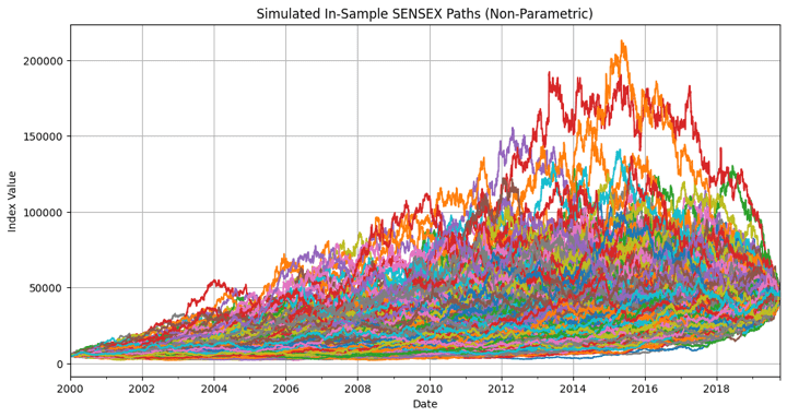
The above graph shows that the starting and ending prices are the same for all 1,000 simulated paths. We should note one thing here. Since we are working with data from a broad market index, whose levels depend on many interlinked macroeconomic variables and factors, it's highly unlikely that the index would have traversed most of the paths simulated above, given the same macroeconomic events that occurred during the simulation period. We are making an implicit assumption here that the specified macroeconomic variables and factors differ in each of the simulated paths, and the interactions between these variables and factors result in the simulated levels that we generate. This holds for any other asset class or asset you decide to replace the SENSEX index with, for retrospective simulation purposes.
Exponential Moving Average Crossover Strategy Development and Backtesting on In-Sample Data, and Parameter Optimisation
Next, we develop a simple trading strategy and conduct a backtest using the in-sample data. The strategy is a simple exponential moving average crossover strategy, where we go long when the short-period exponential moving average (SEMA) of the close price goes above the long-period exponential moving average (LEMA), and we go short when the SEMA crosses the LEMA from above (read more).
Through optimisation, we’ll attempt to find the best SEMA and LEMA combination that yields the maximum returns. For the SEMA, I use lookback periods of 5, 10, 15, 20, … up to 100, and for the LEMA, 20, 30, 40, 50, … up to 300.
The condition is that for any given SEMA and LEMA combination, the LEMA lookback period should be greater than the corresponding SEMA lookback period. We would perform backtests on all different combinations of these SEMA and LEMA values and choose the one that yields the best performance.
We’ll plot:
- the equity curve of the strategy with the best-performing SEMA and LEMA lookback values, plotted against the buy-and-hold equity,
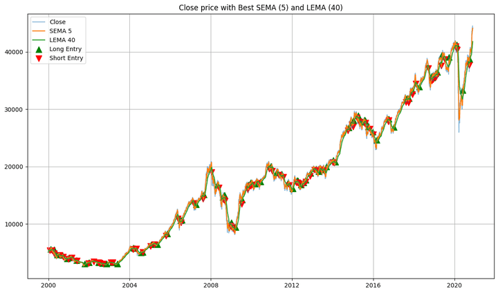
- the buy and sell signals plotted along with the close prices of the in-sample data and the SEMA and LEMA lines,
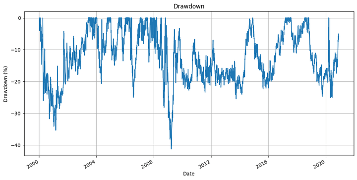
- the underwater plot of the strategy, and,
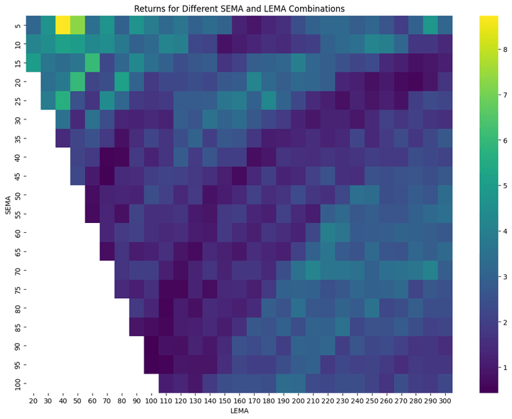
- a heatmap of the returns for different LEMA and SEMA calculations.
We’ll calculate:
- the SEMA and LEMA lookback values for the best-performing combination,
- the total returns of the strategy,
- the maximum drawdown of the strategy, and,
- the Sharpe ratio of the strategy.
We will also review the top 10 SEMA and LEMA combinations and their respective performances.
Here’s the code for all of the above:
And here are the outputs of the above code:
Best SEMA: 5, Best LEMA: 40
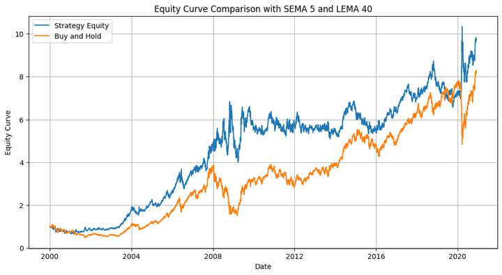
Total Return: 873.43%
Maximum Drawdown: -41.28 %
Sharpe Ratio: 0.59
Top 10 Parameter Combinations:
SEMA  LEMA    Return
2       5    40  8.734340
3       5    50  7.301270
62     15    60  6.021219
89     20    50  5.998316
116    25    40  5.665505
31     10    40  5.183363
92     20    80  5.071913
32     10    50  5.022373
58     15    20  4.959147
27      5   290  4.794400
The heatmap shows a gradual change in color from one adjacent cell to the next. This suggests that slight modifications to the EMA values don’t lead to drastic changes in the strategy's performance. Of course, it would be more gradual if we were to reduce the spacing between the SEMA values from 5 to, say, 2, and between the LEMA values from 10 to, say, 3.
The strategy outperforms the buy-and-hold strategy, as shown in the equity plot. Good news, right? Note here that this was in-sample backtesting. We ran the optimisation on a given dataset, took some information from it, and applied it to the same dataset. It’s like using the prices for the next year (which are unknown to us now, except if you’re time-travelling!) to predict the prices over the next year. However, we can utilise the information gathered from this dataset to apply it to another dataset. That is where we use the out-of-sample data.
Backtesting on Out-of-Sample Data
Let’s run the backtest on the out-of-sample dataset:
Before we see the outputs of the above codes, let’s list what we are doing here.
We are plotting:
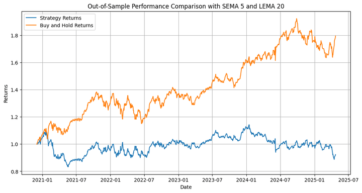
- The equity curve of the strategy plotted alongside that of the buy-and-hold, and,
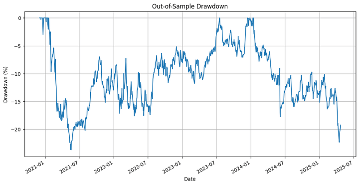
- The underwater plot of the strategy.
We are calculating:
- Strategy returns,
- Buy-and-hold returns,
- Strategy maximum drawdown,
- Strategy Sharpe ratio,
- Buy-and-hold Sharpe ratio, and,
- Strategy hit ratio.
For the Sharpe ratio calculations, we assume a risk-free rate of return of 0. Here are the outputs:
Out-of-Sample Strategy Total Return: 15.46%
Out-of-Sample Buy-and-Hold Total Return: 79.41%
Out-of-Sample Strategy Maximum Drawdown: -15.77 %
Out-of-Sample Strategy Sharpe Ratio: 0.30
Out-of-Sample Buy-and-Hold Sharpe Ratio: 0.56
Out-of-Sample Hit Ratio: 53.70%
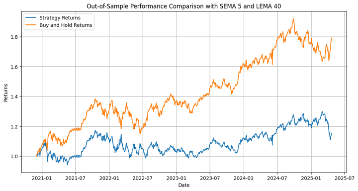

The strategy underperforms the underlying by a significant margin. But that’s not what we're primarily interested in, as far as this blog is concerned. We need to consider that we ran an optimisation on only one of the many paths that the prices could have taken during the in-sample period, and then extrapolated that to the out-of-sample backtest. This is where we use the simulation we performed at the beginning. Let’s run the backtest on the different simulated paths and check the results.
Backtesting on Simulated Paths and Optimising to Extract the Best Parameters
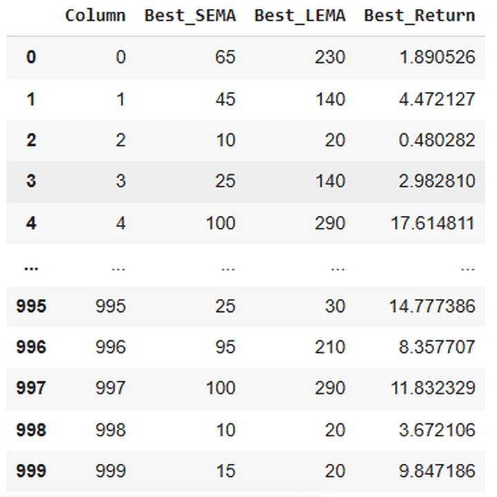
This would keep printing the corresponding SEMA and LEMA values for the best strategy performance, and the performance itself for the simulated paths:
Completed optimization for column 0: SEMA=65, LEMA=230, Return=1.8905
Completed optimization for column 1: SEMA=45, LEMA=140, Return=4.4721
.....................................................................
Completed optimization for column 998: SEMA=10, LEMA=20, Return=3.6721
Completed optimization for column 999: SEMA=15, LEMA=20, Return=9.8472
Here’s a snap of the output of this code:
Now, we’ll sort the above table so that the SEMA and LEMA combination with the best returns for the most paths is at the top, followed by the second-best combination, and so on.
Let’s check how the table would look:
Here’s a snapshot of the output:
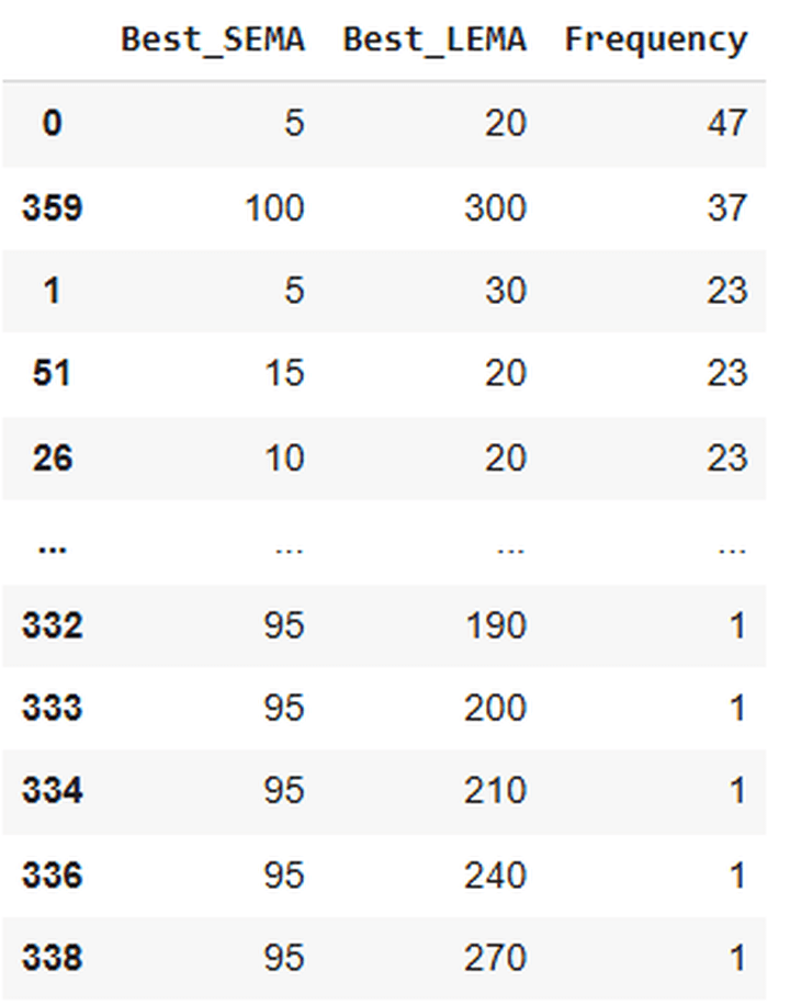
Of the 1000 paths, 47 showed the best returns with a combination of SEMA 5 and LEMA 20. Since I didn’t use a random seed while generating the simulated paths, you can run the code multiple times and obtain different outputs or results. You’ll see that the best SEMA and LEMA combination in the above table would most likely be 5 and 20. The frequencies can change, though.
How do I know?
Because I’ve done so, and have gotten the combination of 5 and 20 in the first place every time (followed by 100 and 300 in the second place). Of course, it’s not that there’s a zero chance of getting some other combination in the top row.
Out-of-Sample Backtesting using Optimised Parameters based on Simulated Data Backtesting
We’ll extract the SEMA and LEMA look-back combination from the previous step that yields the best returns for most of the simulated paths. We’ll use a dynamic approach to automate this selection. Thus, if instead of 5 and 20, we were to obtain, say, 90 and 250 as the optimal combination, the same would be selected, and the backtest would be performed using that.
Let’s use this combination to run an out-of-sample backtest:
Here are the outputs:
Out-of-Sample Strategy Total Return: -7.73%
Out-of-Sample Buy-and-Hold Total Return: 79.41%
Out-of-Sample Strategy Maximum Drawdown: -23.70 %
Out-of-Sample Strategy Sharpe Ratio: -0.05
Out-of-Sample Buy-and-Hold Sharpe Ratio: 0.56
Out-of-Sample Hit Ratio: 52.50%
Discussion on the Results and the Approach
Here, the strategy not only underperforms the underlying but also generates negative returns. So what’s the point of all this effort that we put in? Let’s note that I employed the moving average crossover strategy to illustrate the application of retrospective simulation using a modified Brownian bridge. This approach is more suitable for testing complex strategies with multiple conditions, and machine learning (ML)-based and deep learning (DL)-based strategies.
We have approaches such as walk-forward optimisation and cross-validation to overcome the problem of optimising or fine-tuning a strategy or model on only one of the many possible traversable paths.
However, this approach of retrospective simulation ensures that you don’t have to rely on only one path but can employ multiple retrospective paths. However, since running an ML-based strategy on these simulated paths would be too computationally intensive for most of our readers who don’t have access to GPUs or TPUs, I chose to work with a simple strategy.
Additionally, if you wish to modify the approach, I have included some suggestions at the end.
Evaluation of VaR and C-VaR
Let’s move on to the next part. We’ll utilise the retrospective simulation to calculate the value at risk and the conditional value at risk (read more: 1, 2, 3).
Output:
Value at Risk - 90%: -0.014976172535594811
Value at Risk - 95%: -0.022113806787530325
Value at Risk - 99% -0.04247765359038646
Expected Shortfall - 90%: -0.026779592114352924
Expected Shortfall - 95%: -0.035320511964199504
Expected Shortfall - 99% -0.058565593363193474
Let’s decipher the above output. We first calculated the daily percent returns of all 1000 simulated paths. Every path has 5,155 days of data, which yielded 5,154 returns per path. When multiplied by 1,000 paths, this resulted in 5,154,000 values of daily returns. We used all these values and found the lowest 90th, 95th, and 99th percentile values, respectively.
From the above output, for example, we can say with 95% certainty that if the future prices follow paths similar to these simulated paths, the maximum drawdown that we can face on any given day would be 2.21%. The expected drawdown would be 3.53% if that level gets breached.
Let’s talk about the extremes now. Let’s compare the maximum and minimum daily returns of the simulated paths and the realised in-sample path.
Realized Lowest Daily Return: -0.1315258002691394
Realized Highest Daily Return: 0.17339334818061447
The maximum values from both approaches are close, at around 17.4%. Same for the minimum values, at around -13.2%. This makes a case for using this approach in financial modelling.
Distribution of Simulated Data
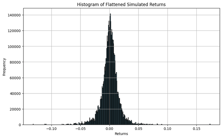
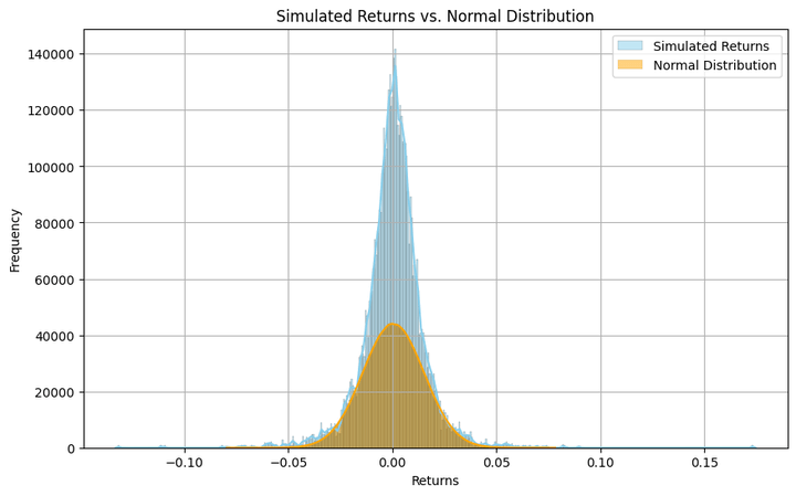
Let’s see how the simulated returns are distributed and compare them visually to a normal distribution. We’ll also calculate the skewness and the kurtosis.
Skewness: -0.11595652411010503
Kurtosis: 9.597364213156881
The argument ‘kde’, when set to ‘True’, smooths the histogram curve, as shown in the above plot. Also, if you want a more granular (coarse) visual of the distribution, you can increase (reduce) the value in the ‘bins’ argument.
Though the histogram resembles a bell curve, it’s far from a normal distribution. It exhibits heavy kurtosis, meaning there are significant chances of finding returns that are many standard deviations away from the mean. And this isn’t any surprise, since that’s how equity and equity-index returns are inherently.
Where This Approach Can Be Most Useful
While the strategy I used here is simple and illustrative, this retrospective simulation framework comes into its own when applied to more complex or nuanced strategies. It’s beneficial in cases where:
- You're testing multi-condition or ML-based models that might overfit on a single realized path.
- You want to stress test a strategy across alternate historical realities that didn’t happen, but very well could have.
- Traditional walk-forward or cross-validation techniques don’t seem to be enough, and you want an added lens to evaluate generalisability.
- You're exploring how a strategy might behave (or might have behaved had the price taken on any alternate price path) under extreme market moves that aren’t present in the actual historical path (but could well have).
In essence, this method enables you to shift your paradigm from “what happened” to “what could have happened,” a subtle yet impactful change in approach.
Suggested Next Steps
If you found this approach interesting, here are a few ways you can extend it:
- Try more sophisticated strategies: Apply this retrospective simulation to mean-reversion, volatility breakout, or reinforcement learning-based strategies.
- Introduce macro constraints: Anchor the simulations around known macroeconomic markers or regime changes to test how strategies behave in such environments.
- Use intermediate anchor points: Instead of just fixing the start and end prices, try anchoring the simulation at quarterly or annual levels to better control drift and convergence.
- Train ML models on simulated paths: If you’re working with supervised learning or deep learning models, train them on multiple simulated realities instead of one.
- Portfolio-level testing: Use this framework to evaluate VaR, CVaR, or stress-test an entire portfolio, not just a single strategy.
This is just the beginning, and how you build on it depends on your curiosity, computing resources, and the questions you're trying to answer.
In Summary
- We introduced a retrospective simulation framework using a non-parametric Brownian bridge approach to simulate alternate historical price paths.
- We employed a simple EMA crossover strategy to illustrate how this simulation can be integrated into a traditional backtesting loop.
- We extracted the best SEMA and LEMA combinations after running backtests on the simulated in-sample paths, and then used those for backtesting on the out-of-sample data.
- This simulation method enables us to test how strategies would behave not only in response to what happened, but also in response to what could have happened, helping us avoid overfitting and uncover robust signals.
- The same simulated paths can be used to derive distributional insights, such as tail risk (VaR, CVaR) or return extremes, offering a deeper understanding of the strategy’s risk profile.
Frequently Asked Questions
1. Curious why we simulate price paths at all?
Real market data shows only one path the market took, among many possible paths. But what if we want to understand how our strategy would behave across many plausible realities in the future, or would have behaved across such realities in the past? That’s why we use simulations.
2. What exactly is a Brownian bridge, and why was it used?
A Brownian bridge simulates price movements that start and end at specific values, like real historical prices. This helps ensure simulated paths are anchored in reality while still allowing randomness in between. The main question we ask here is “What else could have happened in the past?”.
3. How many simulated paths should I generate to make this analysis meaningful?
We used 1000 paths. As mentioned in the blog, when the number of simulated paths increases, computation time increases, but our confidence in the results grows too.
4. Is this only for simple strategies like moving averages?
Not at all. We used the moving average crossover just as an example. This framework can be (and should be) used when you’re testing complex, ML-based, or multi-condition strategies that may overfit to historical data.
5. How do I find the best parameter settings (like SEMA/LEMA)?
For each simulated path, we backtested different parameter combinations and recorded the one that gave the highest return. By counting which combinations performed best across most simulations, we identified the combination that is most likely to perform well. The idea is not to rely on the combination that works on just one path.
6. How do I know which parameter combo to use in the markets?
The idea is to pick the combo that most frequently yielded the best results across many simulated realities. This helps avoid overfitting to the single historical path and instead focuses on broader adaptability. The principle here is not to let our analysis and backtesting be subject to chance or randomness, but rather to have some statistical significance.
7. What happens after I find that "best" parameter combination?
We run an out-of-sample backtest using that combination on data the model hasn’t seen. This tests whether the strategy works outside of the data on which the model is trained.
8. What if the strategy fails in the out-of-sample test?
That’s okay, and in this example, it did! The point is not to "win" with a basic strategy, but to show how simulation and robust testing reveal weaknesses before real money is involved. Of course, when you backtest an actual alpha-generating strategy using this approach and still get underperformance in the out-of-sample, it likely means that the strategy isn’t robust, and you’ll need to make changes to the strategy.
9. How can I use these simulations to understand potential losses?
We followed the approach of flattening the returns from all simulated paths into one big distribution and calculating risk metrics like Value at Risk (VaR) and Conditional VaR (CVaR). These show how bad things can get, and how often.
10. What’s the difference between VaR and CVaR?
- VaR tells us the worst expected loss at a given confidence level (e.g., “you’ll lose no more than 2.2% on 95% of days”).
- CVaR goes a step further and says, “If you lose more than that, here’s the average of those worst days.”.
11. What did we learn from the VaR/CVaR results in this example?
We saw that 99% of days resulted in losses no worse than ~4.25%. But when losses exceeded that threshold, they averaged ~5.86%. That’s a useful insight into tail risk. These are the rare but severe events that can highly affect our trading accounts if not accounted for.
12. Are the simulated return extremes realistic compared to real markets?
Yes, they matched very closely with the maximum and minimum daily returns from the real in-sample data. This validates that our simulation isn’t just random but is grounded in reality.
13. Do the simulated returns follow a normal distribution?
Not quite. The returns showed high kurtosis (fat tails) and slight negative skewness, meaning extreme moves (both up and down) are more common than a normal distribution would have. This mirrors real market behaviour.
14. Why does this matter for risk management?
If our strategy assumes normal returns, we’re heavily underestimating the probability of significant losses. Simulated returns reveal the true nature of market risk, helping us prepare for the unexpected.
15. Is this just an academic exercise, or can I apply this practically?
This approach is incredibly useful in practice, especially when you’re working with:
- Machine learning models that are prone to overfitting
- Strategies designed for high-risk environments
- Portfolios where stress testing and tail risk are crucial
- Regime-switching or macro-anchored models
It helps shift our mindset from "What worked before?" to “What would have worked across many alternate market scenarios?”, and that can be one latent source of alpha.
Conclusion
Hope you learned at least one new thing from this blog. If so, do share what it is in the comments section below and let us know if you’d like to read or learn more about it. The key takeaway from the above discussion is the importance of performing simulations retrospectively and applying them to financial modelling. Apply this approach to more complex strategies and share your experiences and findings in the comments section. Happy learning, happy trading 🙂
Credits
José Carlos Gonzáles Tanaka and Vivek Krishnamoorthy, thank you for your meticulous feedback; it helped shape this article!
Chainika Thakar, thanks for rendering and publishing this, and making it available to the world, that too on your birthday!
Disclaimer: All investments and trading in the stock market involve risk. Any decision to place trades in the financial markets, including trading in stock or options or other financial instruments is a personal decision that should only be made after thorough research, including a personal risk and financial assessment and the engagement of professional assistance to the extent you believe necessary. The trading strategies or related information mentioned in this article is for informational purposes only.