Building a Robust Portfolio with Risk Parity

By Mohak Pachisia

TL;DR

Most investors focus on picking stocks, but asset allocation, how you distribute your investments, matters even more. While poor allocation can cause concentrated risks, a methodical approach to allocation would lead to a more balanced portfolio, better aligned with the portfolio objective.

This blog explains why Risk Parity is a powerful strategy. Unlike equal-weighting or mean-variance optimisation, Risk Parity allocates based on each asset’s risk (volatility), aiming to balance the portfolio so that no single asset dominates the risk contribution.

A practical Python implementation shows how to build and compare an Equal-Weighted Portfolio vs. a Risk Parity Portfolio using the Dow Jones 30 stocks.

Key results:

• Risk Parity outperforms with higher annualized return (15.6% vs. 11.5%), lower volatility (9.9% vs. 10.7%), better Sharpe ratio (1.57 vs. 1.07), and smaller max drawdown (-4.8% vs. -5.8%).
• While compelling, Risk Parity depends on historical volatility, it needs frequent rebalancing, and may underperform in certain market conditions.

To get the most out of this blog, it’s helpful to be familiar with a few foundational concepts.

---

Pre-requisites

First, a solid understanding of Python fundamentals is essential. This includes working with basic programming constructs as well as libraries frequently used in data analysis. You can explore these concepts in-depth through Basics of Python Programming.

Since the blog builds on financial data handling, you’ll also need to be comfortable with stock market data analysis. This involves learning how to obtain market datasets, visualise them effectively, and perform exploratory analysis in Python. For this, check out Stock Market Data: Obtaining Data, Visualization & Analysis in Python.

By covering these prerequisites, you’ll be well-prepared to dive into the concepts discussed in this blog and apply them with confidence.

---

Table of contents

• What is Asset Allocation?
• How Can We Solve This Allocation Imbalance?
• Risk Parity Allocations Process in Python
• Frequently Asked Questions
• A Note on Limitations

---

Ever wondered where your portfolio's risk is coming from?

Most investors focus heavily on picking the right stocks or funds, but what if the way you allocate your capital is more important than the assets themselves? Research consistently shows that asset allocation is the key driver of long-term portfolio performance. For example, Vanguard has published multiple papers reinforcing that asset allocation is the dominant factor in portfolio performance.

In this post, we take a closer look at Risk Parity, a smart and systematic approach to portfolio construction that aims to balance risk, not just capital. Instead of letting one asset class dominate your portfolio's risk, Risk Parity spreads exposure more evenly, potentially leading to greater stability across market cycles.

Quantitative Portfolio Management is a 3-step process.

1. Asset selection
2. Asset Allocation
3. Portfolio rebalance and monitoring

In modern portfolio theory, research has shown that “Asset Allocation” has played a major role in portfolio performance. We will understand Asset Allocation in-depth and then move to understanding one of the possible ways to allocate assets, the Hierarchical Risk Parity method.

---

What is Asset Allocation?

Let us take an example of a novice investor. This investor has a portfolio of 5 stocks and has invested $30,000 in them.

How he/she bought specific proportions of the stocks could depend on subjective analysis or on the funds they have now to buy shares. And this leads to a random exposure of different stocks. As given below, let’s assume that the novice investor is buying stocks, and this is how the allocation looks:

Note: Some of the numbers below could be approximations, for demonstration purposes.

Stocks	Prices	Shares	Exposure
AAPL	243	8	1944
MSFT	218	20	4366
AMZN	190	19	3610
GOOGL	417	20	8340
NVDA	138	85	11742
		Total	30000

As a result, the proportion of each stock bought would widely vary.

Note: The number of shares is not a whole number. The calculations are approximations only for demonstration purposes.

Stocks	Prices	Shares	Exposure	% weights
AAPL	243	8	1946	6%
MSFT	218	20	4366	15%
AMZN	190	19	3610	12%
GOOGL	417	20	8336	28%
NVDA	138	85	11742	39%
		Total	30000	100%

We clearly see that NVDA has a significantly higher weightage of 39% while APPL has merely a weightage of 6%. There is a great disparity in the allocation of funds across the different stocks.

Case 1: NVDA underperforms; it will have a significant impact on your portfolio. Which could lead to large drawdowns, and this is high idiosyncratic risk.

Case 2: APPL outperforms, due to a much lower weightage of the stock in your portfolio. You won’t benefit from it.

---

How Can We Solve This Allocation Imbalance?

Quantitative Portfolio Managers do not allocate funds based on subjectivity. It is industry practice to adopt logical, tested, and effective ways to do it.

Uneven fund allocation can expose your portfolio to concentrated risks. To address this, several systematic asset allocation strategies have been developed. Let’s explore the most notable ones:

1. Equal Weighting:

Approach: Assigns equal capital to each asset.

Note: The number of shares is not a whole number. The calculations are approximations only for demonstration purposes.

Stocks	Prices	Shares	Exposure	% weights
AAPL	243	24.7	6000	20%
MSFT	218	27.5	6000	20%
AMZN	190	31.6	6000	20%
GOOGL	417	14.4	6000	20%
NVDA	138	43.4	6000	20%
		Total	30000	100%

 

• Pros: Simple, intuitive, and reduces concentration risk.
• Cons: Ignores differences in volatility or asset correlation. May overexpose to riskier assets.

Real world example: MSCI World Equal Weighted Index

2. Mean-Variance Optimisation (MVO)

Approach: Based on Modern Portfolio Theory, it aims to maximise expected return for a given level of risk. Though it looks simple, this approach is followed by several fund managers; its effectiveness comes with periodically rebalancing the portfolio exposures :

1. Expected returns
2. Asset volatilities
3. Covariances between assets

Note: The number of shares is not a whole number. The calculations are approximations only for demonstration purposes.

Stocks	Expected Return (%)	Volatility (%)	Optimised Weight (%)	Exposure ($)	Shares
AAPL	9	22	12%	3600	14.8
MSFT	10	18	18%	5400	24.8
AMZN	11	25	25%	7500	39.5
GOOGL	8	20	15%	4500	10.8
NVDA	13	35	30%	9000	65.2
Total			100%	30000

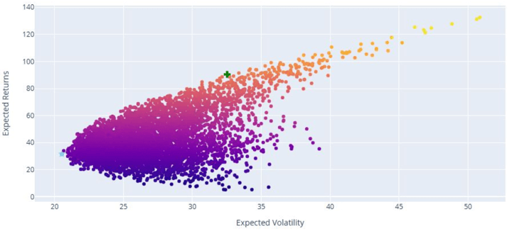
Monte Carlo simulation is often used to test portfolio robustness across different market scenarios. To understand this method better, please read Portfolio Optimisation Using Monte Carlo Simulation.

The plot below shows an example of how portfolios with different expected returns and volatilities are created using the Monte Carlo Simulation method. Thousands, if not more, combinations of weights are considered in this process. The portfolio weights with the highest Sharpe ratio (marked as +) are often taken as the portfolio with the most optimal weightages.

Note: This is only for demonstration purposes, not for stocks used for our example.

• Pros: Theoretically optimal: When inputs are accurate, MVO can construct the most efficient portfolio on the risk-return frontier.
• Cons: Highly sensitive to input assumptions, especially expected returns, which are difficult to forecast.

3. Risk-Based Allocation: Risk Parity

Approach: Instead of allocating capital equally or based on returns, Risk Parity allocates based on risk contribution from each asset. The goal is for each asset to contribute equally to the total portfolio volatility. The process to achieve this includes the following steps.

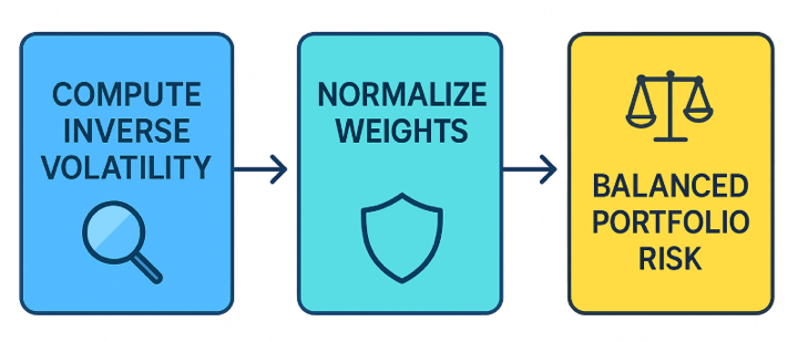
1. Estimate each asset’s volatility
2. Compute the inverse of volatility (i.e., lower volatility → higher weight).
3. Normalise the inverse of volatility to get final weights.

---

What is volatility?

Volatility refers to the degree of variation in the price of a financial instrument over time. It represents the speed and magnitude of price changes, and is often used as a measure of risk.

In simple terms, higher volatility means greater price fluctuations, which can imply more risk or more opportunity.

Formula for Standard Deviation:

$$\sigma = \sqrt{\frac{1}{N-1}\sum_{i=1}^N (r_i - \bar{r})^2}$$

\[ \begin{aligned} \text{where,} \\ &\bullet \ \sigma = \text{Standard deviation} \\ &\bullet \ r_i = \text{Return at time } i \\ &\bullet \ \bar{r} = \text{Average return} \\ &\bullet \ N = \text{Number of periods} \end{aligned} \]

Inverse of Volatility:

The inverse of volatility is simply the reciprocal of volatility. It is often used as a measure of risk-adjusted exposure or to allocate weights inversely proportional to risk in portfolio construction.

σ=Volatility

Then the Inverse of Volatility is:  1/σ

Normalise the inverse of volatility to get final weights :

To determine the final portfolio weights, we take the inverse of each asset's volatility and then normalise these values so that their sum equals 1. This ensures assets with lower volatility receive higher weights while maintaining a fully allocated portfolio.

\[ w_i = \frac{\tfrac{1}{\sigma_i}}{\sum_{j=1}^N \tfrac{1}{\sigma_j}} \] $$ \text{Where,} \\ \bullet \ w_i \quad \text{= weight of asset $i$ in the portfolio} \\ \bullet \ \sigma_i \quad \text{= volatility (standard deviation of returns) of asset $i$} \\ \bullet \ N \quad \text{= total number of assets in the portfolio} \\ \bullet \ \sum_{j=1}^N \tfrac{1}{\sigma_j} \quad \text{= sum of the inverse volatilities of all assets} $$

Example of Risk Parity weighted approach(applying the above approach):

The number of shares is not a whole number. The calculations are approximations only for demonstration purposes.

Stocks	Prices	Volatility (%)	1 / Volatility	Risk Parity Weight (%)	Exposure ($)	Shares
AAPL	243	24	0.0417	18.50%	5,550	22.8
MSFT	218	20	0.05	22.20%	6,660	30.6
AMZN	190	18	0.0556	24.60%	7,380	38.8
GOOGL	417	28	0.0357	15.80%	4,740	11.4
NVDA	138	30	0.0333	18.90%	5,670	41.1
Total				100%	30,000

Result: No single asset dominates the portfolio risk.

Note:

• Volatility is an example based on an assumed % standard deviation.
• “Risk Parity Weight” is proportional to 1 / volatility, normalised to 100%.
  The exposure is calculated as: Risk Parity Weight × Total Capital.
• Shares = Exposure ÷ Price.

Pros:

• Does not rely on expected returns.
• Simple, robust, and uses observable inputs.
• Reduces portfolio drawdowns during volatile periods.

Cons:

• May overweight low-volatility assets (e.g., bonds), underweight growth assets.
• Ignores correlations between assets (unlike HRP).

Other Allocation Methods to Know:

Method	Core Idea	Notes
Hierarchical Risk Parity (HRP)	Uses clustering to detect asset relationships and allocates risk accordingly.	Solves problems of MVO like overfitting and instability.
Minimum Variance Portfolio	Allocates to minimise total portfolio volatility.	Can be very conservative — often heavy on low-volatility assets.
Maximum Diversification	Maximises the diversification ratio (return per unit of risk).	Intuitive for reducing dependency on any one asset.
Black-Litterman Model	Enhances MVO by combining market equilibrium with investor views.	Helps stabilise MVO with more realistic inputs.
Factor-Based Allocation	Allocates to risk factors (e.g., value, momentum, low volatility).	Popular in smart beta and institutional portfolios.

---

Risk Parity Allocations Process in Python

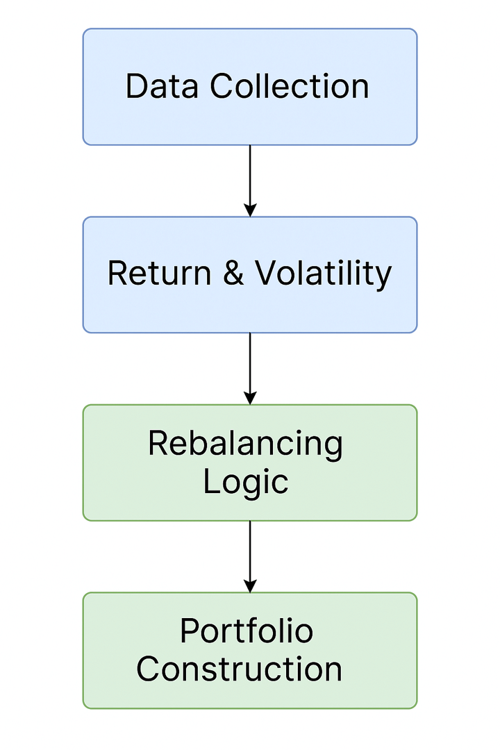
Step 1: Let’s start by importing the relevant libraries

Step 2: We fetch the data for 30 stocks using their Yahoo Finance ticker symbols.

• These 30 stocks are the current 30 constituents of the Dow Jones Industrial Average Index.
• We fetch the data from one month before 2024 begins. And target a window of the entire year 2024. This is done because we use a 20-day rolling period to compute volatilities and rebalance the portfolios. 20 trading days roughly translates to one month.
• Only the “Close” prices are extracted, and the data frame is flattened for further analysis.

Step 3: We create a function to compute the returns of portfolios that are either equally weighted or weighted using the Risk Parity approach.

Purpose: To compute a portfolio's cumulative NAV (Net Asset Value) using equal-weighted or risk-parity rebalancing at fixed intervals.

• price_df: DataFrame containing historical price data of multiple assets, indexed by date.
• rebalance_period (default = 20):
  Number of trading days between each portfolio rebalancing.
• method (default = 'equal'):
  Portfolio weighting method - either 'equal' for equal weights or 'risk_parity' for inverse volatility weights.

Step-by-Step Logic

• Daily Returns Calculation: The function starts by computing daily returns using pct_change() on the price data and dropping the first NaN row.

• Rolling Volatility Estimation: A rolling standard deviation is computed over the rebalance window to estimate asset volatility. To avoid look-ahead bias, this is shifted by one day using .shift(1).

• Start Alignment: The earliest date all rolling volatility is available is identified. The returns and volatility DataFrames are trimmed accordingly.

• NAV Initialisation: A new Series is created to store the portfolio NAV, initialised at 1.0 on the first valid date.

• Rebalance Loop: The function loops through the data in windows of rebalance_period days:

• Volatility and Weights on Rebalance Day: On the first day of each window:

• For 'equal': assigns equal weights to all assets.

• For 'risk_parity': assigns weights inversely proportional to asset volatility.

• Cumulative Returns & NAV Computation: The window’s cumulative returns are calculated and combined with weights to compute the NAV path.

• NAV Normalisation: The NAV is normalised to match the last value of the previous window, ensuring smooth continuity.

Final Output: Returns a time series of the portfolio’s NAV, excluding any missing values.

Step 4: Portfolio Construction

We now proceed to construct two portfolios using the historical price data. This involves calling the portfolio construction function defined earlier. Specifically, we generate:

1. An Equal-Weighted Portfolio, where each asset is assigned the same weight at every rebalancing period.
2. A Risk Parity Portfolio, where asset weights are determined based on inverse volatility, aiming to equalise risk contribution across all holdings.

Both portfolios are rebalanced periodically based on the specified frequency.

Step 5: Portfolio Performance Evaluation

In this step, we evaluate the performance of the two constructed portfolios: Equal-Weighted and Risk Parity, by computing key performance metrics:

• Daily Returns: Calculated from the cumulative NAV series to observe day-to-day performance fluctuations.
• Annualised Return: Derived using the compound return over the entire investment period, scaled to reflect yearly performance.
• Annualised Volatility: Estimated from the standard deviation of daily returns and scaled by the square root of 252 trading days to annualise.
• Sharpe Ratio: A measure of risk-adjusted return, computed as the ratio of annualised return to annualised volatility, assuming a risk-free rate of 0.
• Maximum Drawdown: The maximum observed peak-to-trough decline in portfolio value, indicating the worst-case historical loss.

These metrics offer a comprehensive view of how each portfolio performs in terms of both return and risk. We also visualise the cumulative NAVs of both portfolios to observe their performance trends over time.

---

Frequently Asked Questions

What exactly is Risk Parity?

Risk Parity is a portfolio allocation strategy that assigns weights such that each asset contributes equally to the total portfolio volatility, rather than simply allocating equal capital to each asset. The goal is to prevent any single asset or asset class from dominating the portfolio’s overall risk exposure.

---

How does it differ from Equal Weighting or Mean-Variance Optimisation?

• Equal Weighting: This method allocates the same amount of capital to each asset. It is simple and intuitive, but does not consider the risk (volatility) of each asset, potentially leading to concentrated risk.
• Mean-Variance Optimisation (MVO): Based on Modern Portfolio Theory, MVO seeks to maximise expected return for a given level of risk by considering expected returns and covariances. However, it is highly sensitive to the accuracy of input forecasts.
• Risk Parity: Instead of focusing on returns or allocating equal capital, Risk Parity adjusts weights based on the volatility of each asset, allocating more capital to lower-volatility assets to equalise their risk contributions.

---

Why is asset allocation so important?

Research has shown that asset allocation is the primary driver of long-term portfolio returns, far more significant than selecting individual securities. A well-thought-out allocation helps manage risk and enhances the likelihood of meeting investment goals.

---

How is volatility calculated in Risk Parity?

Volatility is typically measured as the standard deviation of past returns over a rolling window (for example, a 20-day rolling standard deviation). In Risk Parity, assets with lower volatility are assigned higher weights to balance their contribution to total portfolio risk.

---

Is there Python code to implement this?

Yes. The blog provides complete Python code examples using libraries such as pandas for data handling, yfinance for fetching historical prices, and custom functions to rebalance portfolios either by equal weights or by inverse volatility (Risk Parity).

---

Does Risk Parity always outperform other strategies?

No. While Risk Parity often leads to more stable performance and better risk-adjusted returns, especially in diversified or volatile markets, it may underperform simpler strategies like Equal-Weighted portfolios during strong bull markets that favour high-risk assets.

---

What are the limitations of Risk Parity?

• It relies on the historical volatility to set target weights, which may not accurately reflect  the future behaviour of assets, especially during abrupt changes or crises.
• It typically requires frequent rebalancing, which can increase transaction costs and potential slippage.
• It may under-allocate to high-growth assets in trending markets, limiting upside in strong rallies.

---

Are there more advanced methods beyond standard Risk Parity?

Yes. For example, Hierarchical Risk Parity (HRP) uses clustering to understand asset relationships and aims to allocate risk more efficiently by addressing some of the weaknesses of traditional mean-variance approaches, such as instability due to input sensitivity.

---

Conclusion

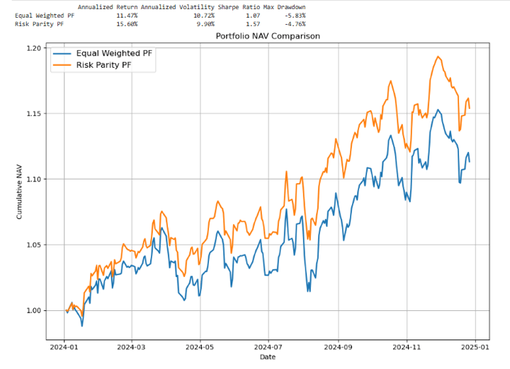
The comparative analysis highlights the clear advantages of using a Risk Parity approach over a traditional Equal-Weighted portfolio. While both portfolios deliver positive returns, Risk Parity stands out with:

• Higher Annualised Return (15.60% vs. 11.47%)
• Lower Volatility (9.90% vs. 10.72%)
• Superior Risk-Adjusted Performance, as seen in the Sharpe Ratio (1.57 vs. 1.07)
• Smaller Max Drawdown (-4.76% vs. -5.83%)

These results demonstrate that by aligning portfolio weights with asset risk (rather than capital), the Risk Parity portfolio may enhance return potential along with better downside protection and smoother performance over time.

The NAV chart further reinforces this conclusion, showing a more consistent and resilient growth trajectory for the Risk Parity strategy.

In summary, for investors prioritising stability over growth, Risk Parity offers a compelling alternative to conventional allocation methods.

---

A Note on Limitations

Although the Risk Parity portfolio delivered stronger returns during the period taken in our example, its performance advantage is not assured in every market phase. Like any strategy, Risk Parity comes with limitations. It relies heavily on historical volatility estimates, which may not always accurately reflect future market conditions, especially during sudden regime shifts or extreme events.

It tends to shine in portfolios that mix high‑ and low‑volatility assets, like stocks and bonds, where equal capital allocation would otherwise concentrate risk.However, if low‑volatility assets underperform or if all assets have similar risk profiles,

Additionally, the strategy often requires frequent rebalancing, which can increase transaction costs and introduce slippage. In strong directional markets, particularly those favouring higher-risk assets, simpler strategies like Equal-Weighted may outperform due to their greater exposure to momentum.

Hence, while Risk Parity provides a systematic way to balance portfolio risk, it should be used with an understanding of its assumptions and practical limitations.

---

Next Steps:

After reading this blog, you may want to enhance your understanding of portfolio design and explore techniques that provide more structure to risk-return trade-offs.

A good place to begin is with Portfolio Variance/Covariance Analysis, which explains how asset correlations impact portfolio volatility. This will provide you with the foundation to understand why diversification works and where it doesn’t.

From there, Portfolio Optimisation Using Monte Carlo Simulation introduces a more dynamic approach. By running thousands of simulated outcomes, you can test how different allocations behave under uncertainty and identify combinations that balance risk and reward.

To round it off, Portfolio Optimisation Methods walks through a range of optimisation frameworks, covering classical mean-variance models as well as alternative methods, so you can compare their strengths and apply them in different market conditions.

Working through these next steps will equip you with practical techniques to analyse, simulate, and optimise portfolios, a skill set that’s critical for anyone looking to manage capital with confidence.

You can explore all of these in detail in the Portfolio Management & Position Sizing Learning Track, which includes the Quantitative Portfolio Management course for a comprehensive understanding of portfolio construction and optimisation.

For those looking to expand beyond portfolio theory into the broader realm of systematic trading, check the Executive Programme in  Algorithmic Trading - EPAT. Its comprehensive curriculum, led by top faculty like Dr. Ernest P. Chan, offers a leading Python algorithmic trading course for career growth. EPAT covers core trading strategies that can be adapted and extended to High-Frequency Trading. Get personalised support for specialising in trading strategies with live project mentorship.

Disclaimer: This blog post is for informational and educational purposes only. It does not constitute financial advice or a recommendation to trade any specific assets or employ any specific strategy. All trading and investment activities involve significant risk. Always conduct your own thorough research, evaluate your personal risk tolerance, and consider seeking advice from a qualified financial professional before making any investment decisions.