By Ishan Shah
Say you're looking at two funds side by side. Both trade in the US, but they're built in very different ways. The first, XYLD, owns the shares in the S&P 500 index. It also sells call options on that index every month. The options bring in a steady fee but give up most big gains. The second fund, DBMF, trades futures on stocks, bonds, currencies and commodities. It tries to copy what a group of managed-futures hedge funds are doing.
We measured both funds over the two years to September 2026. First we scored them with the Sharpe ratio, the most common risk score. It takes the return above cash and divides it by how much the returns swing. On that score, XYLD came out well ahead at about 1.2. DBMF scored a little under 1 on the same test. Then we used the Sortino ratio, which only counts the bad months. This time the two funds were level, both at about 1.8.
So which of the two funds carried more risk? And why would two risk scores disagree about the same funds?
The answer lies in what happened during those two years. The first big fall came in March 2025, when US shares dropped across the board. The second began after the US and Israel struck Iran on 28 February 2026. Oil prices jumped sharply on the next trading day. SPY is a fund that tracks the S&P 500 index. By the end of March, it was nearly 9% below its late-February high. XYLD had its worst months in those two falls. DBMF had losing months too, but most of its biggest months were gains. The Sharpe ratio counts a big gain as risk, just like a big loss. The Sortino ratio doesn't, and that's the only difference between them.
We'll build the Sortino ratio step by step on a small example first. Then we'll come back to these two funds and see where their gap comes from.
We will be covering the following points in this article:
- What is the Sortino ratio?
- What goes into the formula?
- How do you calculate it in Excel?
- How do you calculate the Sortino ratio in Python?
- Why is the Sortino ratio higher than the Sharpe ratio?
- So how do you see what the Sortino ratio adds?
- What happened with XYLD and DBMF?
- What is a good Sortino ratio?
- When does a good Sortino ratio mislead you?
- Three questions to ask of any fund factsheet
- Frequently asked questions
What is the Sortino ratio?
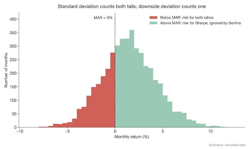
The Sortino ratio measures risk-adjusted return by dividing excess return over a target minimum acceptable return (MAR) by downside deviation. A higher ratio indicates greater return per unit of downside risk.
Introduced by Frank Sortino and Robert van der Meer in 1991, the metric addresses a key limitation of the Sharpe ratio: treating upside volatility as risk. Standard deviation penalizes positive and negative deviations equally, whereas downside deviation focuses solely on shortfalls relative to the target.
For a short definition you can bookmark, see QuantInsti's Sortino ratio glossary entry. It uses the risk-free rate as the target, which is one of the choices we discuss below.
What goes into the formula?
Sortino ratio = (R - T) ÷ DD
- R is the strategy's average return over the period.
- T is the target, also called the minimum acceptable return (MAR).
- DD is the downside deviation of returns below that target.
The top half is your reward: how much you earned above the bar you set. The bottom half is the only risk this ratio cares about.
Which target should you pick? There's no single right answer, and the choice is partly a matter of taste. Many people set the MAR to zero, because they simply don't want to lose money. Others set it to the risk-free rate, which is the return on cash, usually short-term US Treasury bills. They want to beat cash (a choice that matters more when cash pays a few percent a year than when it pays nothing).
How do you calculate it in Excel?
Let's take a made-up strategy with these 12 monthly returns:
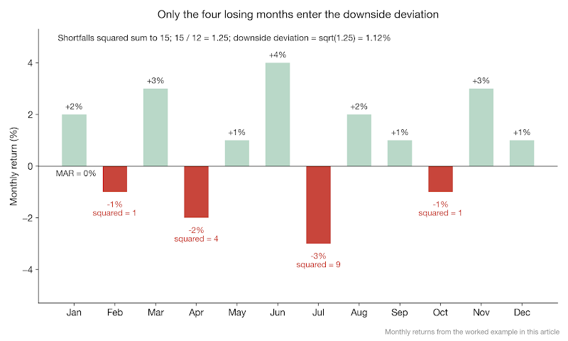
+2%, -1%, +3%, -2%, +1%, +4%, -3%, +2%, +1%, -1%, +3%, +1%
We'll set the MAR to 0%. Put the returns in cells B2:B13 and the MAR in cell E1. Then work across the columns.
Step 1, the shortfalls. In C2, enter =MIN(B2-$E$1, 0) and fill down to C13. Any month that met the target becomes zero. Only four months fell short here: -1%, -2%, -3% and -1%.
Step 2, square them. In D2, enter =C2^2 and fill down. The four squares are 1, 4, 9 and 1, which add up to 15.
Step 3, the downside deviation. In a spare cell, enter =SQRT(AVERAGE(D2:D13)). That averages the squares over all 12 months, zeros included, so you get 15 ÷ 12 = 1.25. Its square root is 1.12%.
This is the step to watch. Some tools divide only by the number of losing months, which is four here. That gives a bigger downside deviation and a smaller ratio. Neither version announces itself, so when you compare Sortino figures from different sources, check which one each source used.
Step 4, the average excess return. Enter =AVERAGE(B2:B13)-E1. The 12 returns add up to +10%, so the average is 0.83% a month.
Step 5, the ratio. Divide step 4 by step 3: 0.83% ÷ 1.12% = 0.75 a month.
A monthly number is hard to compare with anything, so we annualise it. Multiply by the square root of the number of periods in a year, which is =SQRT(12) for monthly data. That gives 0.75 × √12 ≈ 2.58. The square-root rule is a convention and only an approximation. It assumes each month's return has nothing to do with the month before.
By the usual bands, which we'll get to below, 2.58 would count as strong. But it rests on 12 months and just four losing ones, so treat it as an arithmetic example, not a verdict.
How do you calculate the Sortino ratio in Python?
If you'll use this more than once, a short function is cleaner than a spreadsheet. It also copes with thousands of returns without any extra work.
The function gives the same 2.58 as the spreadsheet. Run that check every time you write your own version. A slip in the denominator changes the answer without throwing any error, so a known answer is the only thing that catches it. And if you're judging a strategy, the ratio belongs next to your other numbers when you backtest the strategy.
Why is the Sortino ratio higher than the Sharpe ratio?
Run the Sharpe ratio on the same 12 returns and you get about 1.39. That uses the population standard deviation, to match how we built the downside deviation, and it sets the risk-free rate to zero, so both ratios share the same 0% bar. (With the sample standard deviation, it's 1.33.)
So the Sortino ratio is almost twice the Sharpe ratio here. Does that mean this strategy has lovely big up months? No, and this is where a lot of readers go wrong.
Part of the gap is built in. A risk measure that ignores every month above the target will almost always come out smaller than the standard deviation on a strategy that makes money. A smaller bottom half means a bigger ratio. We checked this with a perfectly symmetric strategy, a normal distribution with the same mean and volatility as our 12 months. Its Sortino ratio is 2.77, about twice its Sharpe ratio, and higher than our example's. So you can't read anything about upside from the gap on one strategy. On the same returns, the Sortino ratio is usually higher than the Sharpe ratio, because its risk measure only looks at the shortfalls. Compare strategies on the same ratio, never one strategy's Sortino against its Sharpe.
So how do you see what the Sortino ratio adds?
You hold the Sharpe ratio fixed and see what happens to the Sortino ratio. Here are two simulated strategies with the same average return, the same volatility and the same Sharpe ratio of 1.11. Strategy A makes a little money almost every month. Then, about once a year, it loses between 4% and 10% in a single month. Strategy B loses a little in four months out of ten. But about once a year, it has a month that's up 4% to 14%.
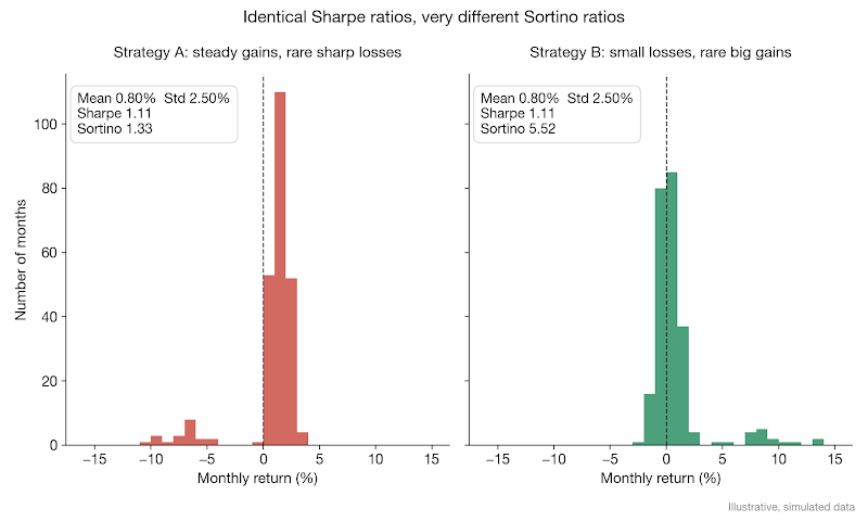
The Sharpe ratio scores them the same. The Sortino ratio gives A 1.33 and B 5.52. If you've ever sat through a month like Strategy A's worst one, you'll probably side with Sortino.
So which number is right? Neither, on its own. Sharpe asks how bumpy the ride was in both directions. Sortino asks how bad the bad months were. When they agree, fine. When two strategies rank in a different order on the two ratios, that tells you their returns are lopsided in different directions. And that's worth knowing before you size a position. For a fuller look at the Sharpe ratio and the related information ratio, read QuantInsti's Sharpe ratio guide. The Sortino ratio also fits into a wider suite of performance and risk metrics.
What happened with XYLD and DBMF?
Real funds are never as tidy as Strategy A and Strategy B, but these two come close. One caution first. We picked this pair and this window after the fact, because they show the effect clearly. That's hindsight. A different pair, or a different two years, could tell a different story.
Here's how we measured them. We took monthly total returns, with distributions reinvested, from October 2024 to September 2026. That's 24 months. For both the risk-free rate and the MAR, we used the monthly return on BIL, a fund that holds one-to-three-month US Treasury bills. It paid between 0.27% and 0.40% a month. Because both ratios use the same rate, their top halves are identical. Any difference between them comes only from the risk measure.
Oct 2024 to Sep 2026, monthly | XYLD | DBMF |
Average return above T-bills | 0.67% | 0.76% |
Standard deviation | 1.94% | 2.75% |
Downside deviation | 1.32% | 1.48% |
Sharpe ratio (annualised) | 1.19 | 0.95 |
Sortino ratio (annualised) | 1.75 | 1.77 |
Months below the T-bill rate | 5 | 9 |
Look at the standard deviation first. DBMF's was about 42% bigger than XYLD's, so the Sharpe ratio marked it down hard. But its downside deviation was only about 12% bigger. Why did the gap shrink so much?
Because DBMF's swings mostly pointed up. Months that beat its own average made up 54% of its variance. February 2026 alone, when it gained 7.8%, supplied a quarter of it. The Sortino ratio ignores all of that. XYLD was the other way round. Its two March selloffs made up 83% of the squared shortfalls behind its downside deviation, so the Sortino ratio counted almost all of its worst swings.
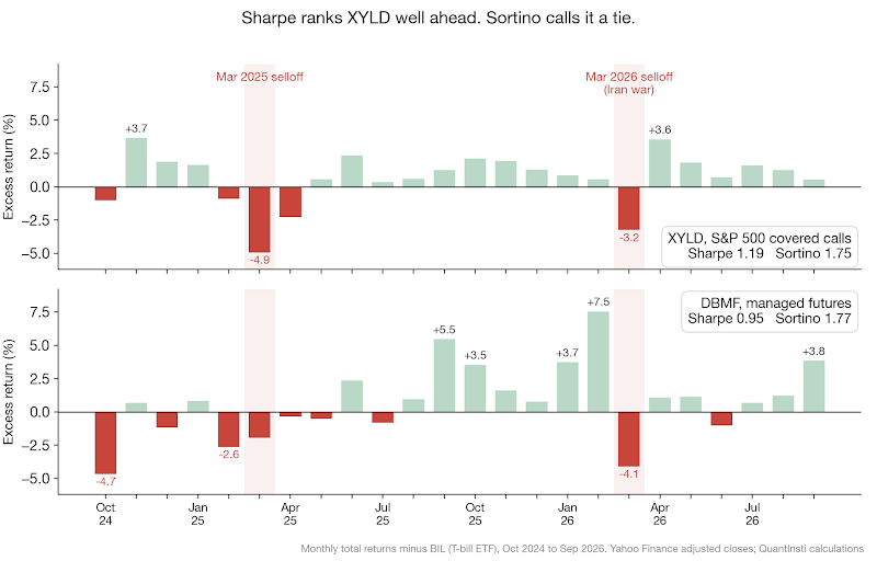
This compares what each ratio measures on two real funds over one window. It isn't a view on either fund, and their past returns don't tell you how they'll behave next.
Did DBMF dodge the Iran selloff, then? No. In March 2026 it lost 3.8%, more than XYLD's 3.0%. The difference comes from the whole two years. DBMF had more losing months, nine against five, and it also had more big winning ones. Selling calls gives away part of the upside, and you can see that in the rebound. From 30 March to 30 April 2026, SPY gained 13.7%, while XYLD gained 5.9%.
What is a good Sortino ratio?
People commonly use these bands:
- Below 0 means the strategy returned less than its target or the risk-free rate, so it didn't clear the bar it set itself.
- Between 0 and 1 is usually called suboptimal, because the downside risk isn't being well rewarded.
- Above 1 is considered good.
- Above 2 is considered very good.
- Above 3 is called excellent, though a number that high deserves a second look at the data before you believe it.
These cut-offs are arbitrary. They're round numbers that stuck, not values anyone worked out. A Sortino ratio only means something in context, because the asset class, the market conditions, the sample length and the MAR all move it.
How much can the window matter? Here's one simulated strategy, measured over rolling 36-month windows. The 36 months is an arbitrary choice too. We picked three years because it's a length people often quote.
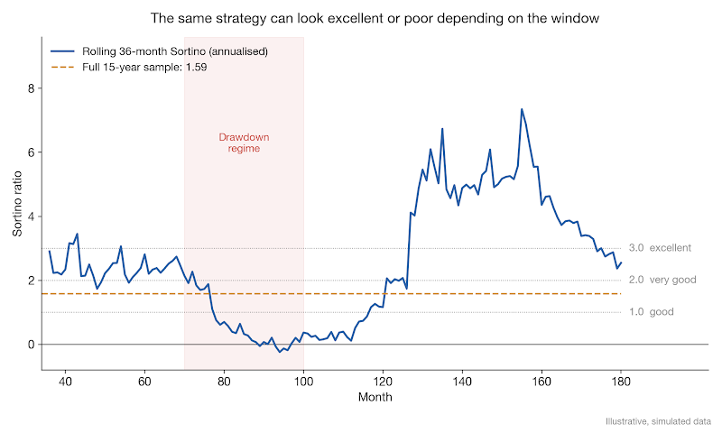
Over the full 15 years, the ratio is 1.59. But depending on which three years you look at, the same strategy scores anywhere from about -0.24 to 7.35. The strategy's rules never changed. What changed was which market conditions, and how many losing months, each window happened to contain.
Our two real funds move with the window as well. Take only the last 12 months, October 2025 to September 2026. XYLD still leads on the Sharpe ratio, 2.43 against 2.10. But now DBMF leads on the Sortino ratio, 4.72 against 3.99. Nothing about either fund changed between the two calculations. We only dropped the first year. And look how high all four numbers are. A calm year with few losing months lifts every score into the "excellent" band.
When does a good Sortino ratio mislead you?
- It only looks backwards. It describes what already happened. It makes no promise about future performance.
- Your MAR choice changes the answer. Move the target and the ratio moves with it. On our two funds, switching the target from the T-bill rate to 0% lifts both Sortino ratios from about 1.75 to about 2.85.
- A strategy with few losing months has a fragile denominator. If there were only a few losing periods in the sample (four, in our worked example), the downside deviation rests on very little data. XYLD shows how far this goes. In the last 12 months, only March 2026 fell below the T-bill rate, so that one month was its whole downside deviation. Over the full two years, take out March 2025 alone and XYLD's Sortino ratio jumps from 1.75 to 3.61.
- It can't see the shape of the tail. A strategy can show a decent Sortino ratio and still carry the risk of a rare, severe loss that just hasn't happened yet (selling options for steady premium is the classic case).
That last point is why the maximum drawdown should sit next to any Sortino ratio you read. The ratio tells you how bad the typical bad month was. The drawdown tells you how bad it got in a row. For more on combining them, see portfolio risk and returns.
Three questions to ask of any fund factsheet
Next time a factsheet shows you a Sortino ratio, ask these three things before you trust it.
- Was it built the same way as the number you're comparing it with? Check the window, the target and whether the downside deviation averages over all months or only the losing ones. If any of those differ, the two numbers can't be ranked.
- Are you comparing Sortino with Sortino? Remember the built-in gap, and never set one fund's Sortino against its own Sharpe. Rank funds on one ratio at a time, and pay attention when two of them swap places between ratios.
- Which months make up the downside deviation? If two or three months supply most of it, ask what the ratio looks like without them.
Put XYLD and DBMF through those three questions and you get the real lesson of the opening example. The Sharpe ratio preferred XYLD. The Sortino ratio called it a tie over two years, then put DBMF ahead over one. And XYLD's score rested on a handful of selloff months. That's what each ratio could see, and it's all this example shows. To try it on your own strategy, run the sortino_ratio function above on its monthly returns and work through the same three questions.
Frequently asked questions
What is the Sortino ratio in simple terms?
The Sortino ratio shows how much return you earned for the bad kind of risk. It takes the return above a chosen target. Then it divides that by the downside deviation, which only looks at returns below the target. Good months don't count as risk. A higher number means more reward per unit of downside.
What is the difference between the Sortino and Sharpe ratios?
The two ratios differ only in the risk they divide by. The Sharpe ratio uses standard deviation, so big gains and big losses both count as risk. The Sortino ratio uses downside deviation, so only shortfalls below a target count. When two funds rank differently on each, their returns are lopsided in different ways.
What is a good Sortino ratio?
Common bands say above 1 is good and above 2 is very good. Above 3 is called excellent. These are round numbers, not tested limits. The same strategy can score very differently over different time windows. So compare similar funds measured over the same period, against the same target.
How do you calculate downside deviation?
Start by subtracting the target return from each period's return. Keep the shortfalls and set every other period to zero. Square the shortfalls and average them over all periods, not just the losing ones. Then take the square root. Some tools divide by the losing periods only, which gives a larger figure.
Can the Sortino ratio be negative?
Yes, it can. A negative Sortino ratio means the average return was below the target over the period. That target is often zero or the risk-free rate. The downside deviation is never negative. So the sign comes from the top half of the formula. A negative score means the strategy missed its own bar.
Is a higher Sortino ratio always better?
Not always. A high score can rest on just a few losing months, and that makes it fragile. It also can't see a rare, severe loss that simply hasn't happened yet. Strategies that sell options for steady income are a common example. That's why it helps to read the maximum drawdown next to it.
Sources
- Sortino, F. A. and van der Meer, R. (1991). Downside Risk. Journal of Portfolio Management, 17(4), 27-31: https://doi.org/10.3905/jpm.1991.409343
- Sortino, F. A. and Price, L. N. (1994). Performance Measurement in a Downside Risk Framework. Journal of Investing, 3(3), 59-64: https://doi.org/10.3905/joi.3.3.59
- Quantra glossary, Sortino Ratio: https://quantra.quantinsti.com/glossary/Sortino-Ratio
- Al Jazeera (2 March 2026). Oil prices rise sharply after US, Israeli attacks on Iran: https://www.aljazeera.com/news/2026/3/2/oil-prices-rise-sharply-after-us-israeli-attacks-on-iran/
- Global X ETFs. S&P 500 Covered Call ETF (XYLD), fund page: https://www.globalxetfs.com/funds/xyld/
- iMGP. DBi Managed Futures Strategy ETF (DBMF), fund page: https://www.imgp.com/us/fund/US53700T8273
- XYLD, DBMF, SPY and BIL daily and monthly total returns, October 2024 to September 2026: Yahoo Finance adjusted closes via yfinance; QuantInsti calculations.
Measuring performance and risk properly is a big part of building strategies that hold up in live markets. QuantInsti's EPAT (Executive Programme in Algorithmic Trading) covers these metrics in depth, as part of a practitioner-led algorithmic trading course that spans strategy design, Python, backtesting and risk management.
If you'd prefer a self-paced start on the coding side, Quantra's Python for trading course covers the data-handling basics behind the Sortino function above.
Disclaimer
This article is for education only. QuantInsti is not registered with SEBI as a Research Analyst or an Investment Adviser, and nothing here is investment advice, a research report or a recommendation to buy, sell or hold any security, fund, index product, currency or crypto asset. Where we name a security, a price or a date, it's there only to illustrate a concept with historical data. It isn't a view on where that price will go.
Past results don't indicate future results, and that applies even more to backtested or simulated results, which are built with hindsight and can leave out costs, slippage and execution limits that change the outcome. Trading involves substantial risk of loss. With leveraged products such as futures, options, CFDs and crypto derivatives, you can lose more than the money you put in.
Do your own research. Before you make any investment or trading decision, consult a SEBI-registered Investment Adviser or Research Analyst who can take your own circumstances into account.