Welcome to the second part of this two-part blog series on the bias-variance tradeoff and its application to trading in financial markets.
In the first part, we attempted to develop an intuition for the bias-variance decomposition. In this part, we’ll extend our learnings from the first part and develop a trading strategy.
Prerequisites
If you have some basic knowledge of Python and ML, you should be able to read and comprehend the article. These are some pre-requisites:
- https://blog.quantinsti.com/bias-variance-machine-learning-trading/
- Linear algebra (basic to intermediate)
- Python programming (basic to intermediate)
- Machine learning (working knowledge of regression and regressor models)
- Time series analysis (basic to intermediate)
- Experience in working with market data and creating, backtesting, and evaluating trading strategies
Also, I have added some links for further reading at relevant places throughout the blog.
If you're new to Python or need a refresher on it, you can start with Basics of Python Programming and then move to Python for Trading: Basic on Quantra for trading-specific applications.
To familiarize yourself with machine learning, and with the concept of linear regression, you can go through Machine Learning for Trading and Predicting Stock Prices Using Regression.
Because the article also covers time series transformations and stationarity, you can familiarize yourself with Time Series Analysis. Knowledge of handling financial market data and practical experience in strategy creation, backtesting, and evaluation will help you apply the article's learnings to your strategies.
In this blog, we’ll cover the complete pipeline for using machine learning to build and backtest a trading strategy while utilising the bias-variance decomposition to select the appropriate prediction model. So, here goes…
The flow of this article is as follows:
- Importing Libraries
- Downloading Data
- Defining Technical Indicators as Predictor Variables
- Defining the Target Variable
- Walk Forward Optimization with PCA and VIF
- Trading Strategy Formulation, Backtesting, and Evaluation
- Calling the Functions Defined Previously
- Bias-Variance Decomposition
- Stationarizing the Inputs
- Running a Prediction using the Chosen Model
- Checking the Trade Logs
- Equity Curves, Sharpe, Drawdown, Hit Ratio, Returns Distribution, Average Returns per Trade, and CAGR
- Some Realistic Considerations
- A Note on the Downloadable Python Notebook
As a ritual, the first step is to import the necessary libraries.
Importing Libraries
If you don’t have any of these installed, a ‘!pip install’ command should do the trick (if you don’t want to leave the Jupyter Notebook environment, or if you want to work on Google Colab).
Downloading Data
Next, we define a function for downloading the data. We’ll use the yfinance API here.
Notice the argument ‘multi_level_index’. Recently (I’m writing this in April 2025), there have been some changes in the yfinance API. When downloading price level and volume data for any security through the specified API, the ticker name of the security gets added as a heading.
It looks like this when downloaded:
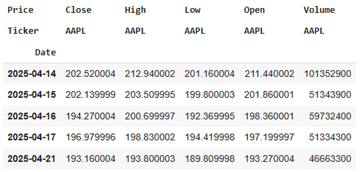
For people (like me!) who are accustomed to not seeing this extra level of heading, removing it while downloading the data is a good idea. So we set the ‘multi_level_index’ argument to ‘False’.
Defining Technical Indicators as Predictor Variables
Next, since we are using machine learning to build a trading strategy, we must include some features (sometimes called predictor variables) on which we train the machine learning model. Using technical indicators as predictor variables is a good idea when trading in the financial markets. Let’s do it now.
Eventually, we’ll see the list of indicators when we call this function on the asset dataframe.
Defining the Target Variable
The next chronological step is to define the target variable/s. In our case, we’ll define a single target variable, the close-to-close 5-day percent return. Let’s see what this means. Suppose today is a Monday, and there are no market holidays, barring the weekends, this week. Consider the percent change in tomorrow’s (Tuesday’s) closing price over today’s closing price, which would be a close-to-close 1-day percent return. At Wednesday’s close, it would be the 2-day percent return, and so on, till the following Monday, when it would be the 5-day percent return. Here’s the Python implementation for the same:
Why do we use the shift(-5) here? Suppose the 5-day percent return based on the closing price of the following Monday over today’s closing price is 1.2%. By using shift(-5), we are placing this value of 1.2% in the row for today’s OHLC price levels, volume, and other technical indicators. Thus, when we feed the data to the ML model for training, it learns by considering the technical indicators as predictors and the value of 1.2% in the same row as the target variable.
Walk Forward Optimization with PCA and VIF
One essential consideration while training ML models is to ensure that they display robust generalization. This means that the model should be able to extrapolate its performance on the training dataset (sometimes called in-sample data) to the test dataset (sometimes called out-of-sample data), and its good (or otherwise) performance should be attributed primarily to the inherent nature of the data and the model, rather than to chance.
One approach towards this is combinatorial purged cross-validation with embargoing. You can read this to learn more.
Another approach is walk-forward optimisation, which we will use (read more: 1 2).
Another essential consideration while building an ML pipeline is feature extraction. In our case, the total predictors we have is 21. We need to extract the most important ones from these, and for this, we will use Principal Component Analysis and the Variance Inflation Factor. The former extracts the top 4 (a value that I chose to work with; you can change it and see how the backtest changes) combinations of features that explain the most variance within the dataset, while the latter addresses mutual information, also known as multicollinearity.
Here’s the Python implementation of building a function that does the above:
Trading Strategy Formulation, Backtesting, and Evaluation
We now come to the meaty part: the strategy formulation. Here are the strategy outlines:
Initial capital: ₹10,000.
Capital to be deployed per trade: 20% of initial capital (₹2,000 in our case).
Long condition: when the 5-day close-to-close percent return prediction is positive.
Short condition: when the 5-day close-to-close percent return prediction is negative.
Entry point: open of day (N+1). Thus, if today is a Monday, and the prediction for the 5-day close-to-close percent returns is positive today, I’ll go long at Tuesday’s open, else I’ll go short at Tuesday’s open.
Exit point: close of day (N+5). Thus, after I get a positive (negative) prediction today and go long (short) during Tuesday’s open, I’ll square off at the closing price of the following Monday (provided there are no market holidays in between).
Capital compounding: no. This means that our profits (losses) from every trade are not getting added (subtracted) to (from) the tradable capital, which remains fixed at ₹10,000.
Here’s the Python code for this strategy:
Next, we define the functions to evaluate the Sharpe ratio and maximum drawdowns of the strategy and a buy-and-hold approach.
Calling the Functions Defined Previously
Now, we begin calling some of the functions mentioned above.
We’ll start with downloading the data using the yfinance API. The ticker and period are user-driven. When running this code, you’ll be prompted to enter the same. I chose to work with the 10-year daily data of the NIFTY-50, the broad market index based on the National Stock Exchange (NSE) of India. You can choose a smaller timeframe; the longer the time frame, the longer it will take for the subsequent codes to run. After downloading the data, we’ll create the technical indicators by calling the ‘create_technical_indicators’ function we defined previously.
Here’s the output of the above code:
Enter a valid yfinance API ticker: ^NSEI
Enter the number of years for downloading data (e.g., 1y, 2y, 5y, 10y): 10y
YF.download() has changed argument auto_adjust default to True
[*********************100%***********************]  1 of 1 completed
Next, we align the data:
Let’s check the two dataframes ‘indicators’ and ‘data_merged’.
RangeIndex: 2443 entries, 0 to 2442
Data columns (total 21 columns):
 #   Column           Non-Null Count  Dtype
---  ------           --------------  -----
 0   sma_5            2443 non-null   float64
 1   sma_10           2443 non-null   float64
 2   ema_5            2443 non-null   float64
 3   ema_10           2443 non-null   float64
 4   momentum_5       2443 non-null   float64
 5   momentum_10      2443 non-null   float64
 6   roc_5            2443 non-null   float64
 7   roc_10           2443 non-null   float64
 8   std_5            2443 non-null   float64
 9   std_10           2443 non-null   float64
 10  rsi_14           2443 non-null   float64
 11  vwap             2443 non-null   float64
 12  obv              2443 non-null   int64
 13  adx_14           2443 non-null   float64
 14  atr_14           2443 non-null   float64
 15  bollinger_upper  2443 non-null   float64
 16  bollinger_lower  2443 non-null   float64
 17  macd             2443 non-null   float64
 18  cci_20           2443 non-null   float64
 19  williams_r       2443 non-null   float64
 20  stochastic_k     2443 non-null   float64
dtypes: float64(20), int64(1)
memory usage: 400.9 KB
Index: 2438 entries, 0 to 2437
Data columns (total 28 columns):
#   Column           Non-Null Count  Dtype
---  ------           --------------  -----
0   Date             2438 non-null   datetime64[ns]
1   Close            2438 non-null   float64
2   High             2438 non-null   float64
3   Low              2438 non-null   float64
4   Open             2438 non-null   float64
5   Volume           2438 non-null   int64
6   sma_5            2438 non-null   float64
7   sma_10           2438 non-null   float64
8   ema_5            2438 non-null   float64
9   ema_10           2438 non-null   float64
10  momentum_5       2438 non-null   float64
11  momentum_10      2438 non-null   float64
12  roc_5            2438 non-null   float64
13  roc_10           2438 non-null   float64
14  std_5            2438 non-null   float64
15  std_10           2438 non-null   float64
16  rsi_14           2438 non-null   float64
17  vwap             2438 non-null   float64
18  obv              2438 non-null   int64
19  adx_14           2438 non-null   float64
20  atr_14           2438 non-null   float64
21  bollinger_upper  2438 non-null   float64
22  bollinger_lower  2438 non-null   float64
23  macd             2438 non-null   float64
24  cci_20           2438 non-null   float64
25  williams_r       2438 non-null   float64
26  stochastic_k     2438 non-null   float64
27  Target           2438 non-null   float64
dtypes: datetime64[ns](1), float64(25), int64(2)
memory usage: 552.4 KB
The dataframe ‘indicators’ contains all 21 technical indicators mentioned earlier.
Bias-Variance Decomposition
Now, the primary purpose of this blog is to demonstrate how the bias-variance decomposition can aid in developing an ML-based trading strategy. Of course, we aren’t just limiting ourselves to it; we are also learning the complete pipeline of creating and backtesting an ML-based strategy with robustness. But let’s talk about the bias-variance decomposition now.
We begin by defining six different regression models:
You can add more or subtract a couple from the above list. The more regressor models there are, the longer the subsequent codes will take to run. Reducing the number of estimators in the relevant models will also result in faster execution of the subsequent codes.
In case you’re wondering why I chose regressor models, it’s because the nature of our target variable is continuous, not discrete. Although our trading strategy is based on the direction of the prediction (bullish or bearish), we are training the model to predict the 5-day return, a continuous random variable, rather than the market movement, which is a categorical variable.
After defining the models, we define a function for the bias-variance decomposition:
You can decrease the value of num_rounds to, say, 10, to make the following code run faster. However, a higher value gives a more robust estimate.
This is a good repository to look up the above code:
https://rasbt.github.io/mlxtend/user_guide/evaluate/bias_variance_decomp/
Finally, we run the bias-variance decomposition:
The output of this code is:
Bias-Variance Decomposition for All Models:
                  Total Error      Bias  Variance  Irreducible Error
LinearRegression     0.000773  0.000749  0.000024      -2.270048e-19
Ridge                0.000763  0.000743  0.000021       1.016440e-19
DecisionTree         0.000953  0.000585  0.000368      -2.710505e-19
Bagging              0.000605  0.000580  0.000025       7.792703e-20
RandomForest         0.000605  0.000580  0.000025       1.287490e-19
GradientBoosting     0.000536  0.000459  0.000077       9.486769e-20
Let’s analyse the above table. We’ll need to choose a model that balances bias and variance, meaning it neither underfits nor overfits. The decision tree regressor best balances bias and variance among all six models.
However, its total error is the highest. Bagging and RandomForest display similar total errors. GradientBoosting displays not just the lowest total error but also a higher degree of variance compared to Bagging and RandomForest; thus, its ability to generalise to unseen data should be better than the other two, since it would capture more complex patterns..
You might be compelled to think that with such proximity of values, such in-depth analysis isn’t apt owing to a high noise-to-signal ratio. However, since we are running 100 rounds of the bias-variance decomposition, we can be confident in the noise mitigation that results.
Long story cut short, we’ll choose to train the GradientBoosting regressor, and use it to predict the target variable. You can, of course, change the model and see how the strategy performs under the new model. Please note that we are treating the ML models as black boxes here, as exploring their underlying mechanisms is outside the scope of this blog. However, when using ML models for any use case, we should always be aware of their inner workings and choose accordingly.
Having discussed all the above, is there a way of reducing the errors of one or more of the above regressor models? Yes, and it’s not a mere technique, but an integral part of working with time series. Let’s discuss this.
Stationarizing the Inputs
We are working with time series data (read more), and when performing financial modeling tasks, we need to check for stationarity (read more). In our case, we should check our input variables (the predictors) for stationarity.
Let’s define a function to check the order of integration of the predictor variables. This function would check whether we need to difference the time series (in our case, the predictor variables) and if so, how many times (read more).
Let’s check the predictor variables for stationarity and apply differencing to the required predictors.
Here’s the code:
Here’s a snapshot of the output of the above code:
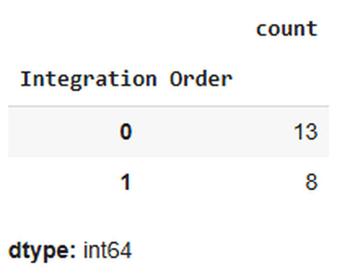
The above output indicates that 13 predictor variables don’t require stationarisation, while 8 do. Let’s stationarise them.
Let’s verify whether the stationarising got done as expected or not:
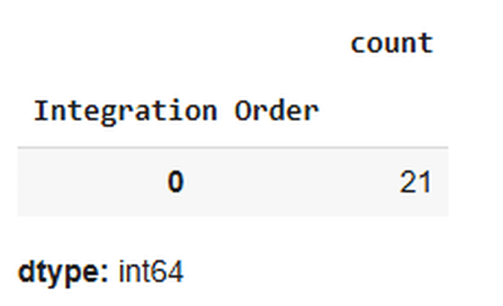
Yup, done!
Let’s align the data again:
Let’s check the bias-variance decomposition of the models with the stationarised predictors:
Here’s the output:
Bias-Variance Decomposition for All Models with Stationarised Predictors:


                  Total Error      Bias  Variance  Irreducible Error
LinearRegression     0.000384  0.000369  0.000015       5.421011e-20
Ridge                0.000386  0.000373  0.000013      -3.726945e-20
DecisionTree         0.000888  0.000341  0.000546       2.168404e-19
Bagging              0.000362  0.000338  0.000024      -1.151965e-19
RandomForest         0.000363  0.000338  0.000024       7.453890e-20
GradientBoosting     0.000358  0.000324  0.000034      -3.388132e-20
There you go. Just by following Time Series 101, we could reduce the errors of all the models. For the same reason that we discussed earlier, we’ll choose to run the prediction and backtesting using the GradientBoosting regressor.
Running a Prediction using the Chosen Model
Next, we run a walk-forward prediction using the chosen model:
Now, we create a dataframe, ‘final_data’, that contains only the open prices, close prices, actual/realised 5-day returns, and 5-day returns predicted by the model. We need the open and close prices for entering and exiting trades, and the predicted 5-day returns, to determine the direction in which we take trades. We then call the ‘backtest_strategy’ function on this dataframe.
Checking the Trade Logs
The dataframe ‘trades_df_differenced’ contains the trade logs.
We’ll convert the decimals of the values in the dataframe for better visibility:
Let’s check the dataframe ‘trades_df_differenced’ now:
Here’s a snapshot of the output of this code:
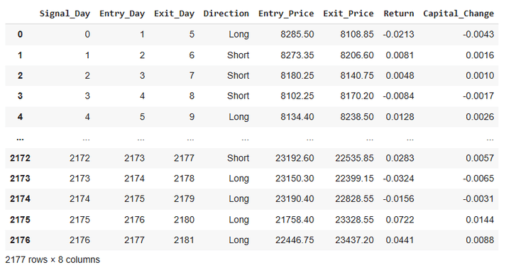
From the table above, it’s apparent that we take a new trade daily and deploy 20% of our tradeable capital on each trade.
Equity Curves, Sharpe, Drawdown, Hit Ratio, Returns Distribution, Average Returns per Trade, and CAGR
Let’s calculate the equity for the strategy and the buy-and-hold approach:
Next, we calculate the Sharpe and the maximum drawdowns:
The above code requires you to input the risk-free rate of your choice. It is typically the government treasury yield. You can look it up online for your geography. I chose to work with a value of 6.6:
Enter the risk-free rate (e.g., for 5.3%, enter only 5.3): 6.6
Now, we’ll reindex the dataframes to a datetime index.
We’ll plot the equity curves next:
This is how the strategy and buy-and-hold equity curves look when plotted on the same chart:
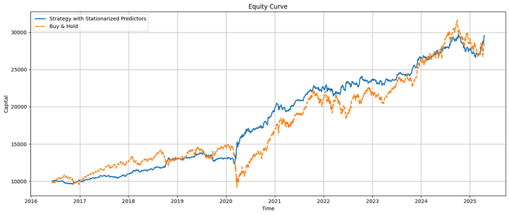
The strategy equity and the underlying move almost in tandem, with the strategy underperforming before the COVID-19 pandemic and outperforming afterward. Toward the end, we’ll discuss some realistic considerations about this relative performance.
Let’s have a look at the drawdowns of the strategy and the buy-and-hold approach:
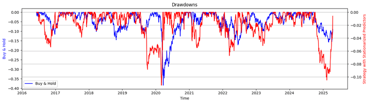
Let’s take a look at the Sharpe ratios and the maximum drawdown by calling the respective functions that we defined earlier:
Output:
Sharpe Ratio (Strategy with Stationarised Predictors):    0.89
Sharpe Ratio (Buy & Hold):  0.42
Max Drawdown (Strategy with Stationarised Predictors):    -11.28%
Max Drawdown (Buy & Hold):  -38.44%
Here’s the hit ratio:
Hit Ratio of Strategy with Stationarised Predictors: 54.09%
This is how the distribution of the strategy returns looks like:
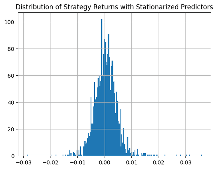
Finally, let’s calculate the average profits (losses) per winning (losing) trade:
Average Profit for Profitable Trades with Stationarised Predictors: 0.0171
Average Loss Loss-Making Trades with Stationarised Predictors: -0.0146
Based on the above trade metrics, we profit more on average in each trade than we lose. Also, the number of positive trades exceeds the number of negative trades. Therefore, our strategy is safe on both fronts. The maximum drawdown of the strategy is limited to 10.48%.
The reason: The holding period for any trade is 5 days, using only 20% of our available capital per trade. This also reduces the upside potential per trade. However, since the average profit per profitable trade is higher than the average loss per loss-making trade and the number of profitable trades is higher than the number of loss-making trades, the chances of capturing more upsides are higher than those of capturing more downsides.
Let’s calculate the compounded annual growth rate (CAGR):
CAGR (Buy & Hold): 13.0078%
CAGR (Strategy with Stationarised Predictors): 13.3382%
Finally, we’ll evaluate the regressor model's accuracy, precision, recall, and f1 scores (read more).
Confusion Matrix (Stationarised Predictors):
 [[387 508]
 [453 834]]
Accuracy (Stationarised Predictors): 0.5596
Recall (Stationarised Predictors): 0.6480
Precision (Stationarised Predictors): 0.6215
F1-Score (Stationarised Predictors): 0.6345
Some Realistic Considerations
Our strategy outperformed the underlying index during the post-COVID-19 crash period and marginally outperformed the overall market. However, if you are thinking of using the skeleton of this strategy to generate alphas, you’ll need to peel off some assumptions and take into account some realistic considerations:
Transaction Costs: We enter and exit trades daily, as we saw earlier. This incurs transaction costs.
Asset Selection: We backtested using the broad market index, which isn’t directly tradable. We’ll need to choose ETFs or derivatives with this index as the underlying. The strategy's performance would also be subject to the inherent characteristics of the asset that we decide to trade as a proxy for the broad market index.
Slippages: We enter our trades at the market's opening and exit at its close. Trading activity can be high during these periods, and we may encounter considerable slippages.
Availability of Partially Tradable Securities: Our backtest implicitly assumes the availability of fractional assets. For example, if our capital is ₹2,000 and the entry price is ₹20,000, we’ll be able to buy or sell 0.1 units of the underlying, ignoring all other costs.
Taxes: Since we are entering and exiting trades within very short time frames, apart from transaction charges, we would incur a significant amount of short-term capital gains tax (STCG) on the profits earned. This, of course, would depend on your local regulations.
Risk Management: In the backtest, we omitted stop-losses and take-profits. You are encouraged to include them and let us know your findings on how the strategy's performance gets modified.
Event-driven Backtesting: The backtesting we performed above is vectorized. However, in real life, tomorrow comes only after today, and we must consider this when performing a backtest. You can explore the Blueshift at https://blueshift.quantinsti.com/ and try backtesting the above strategy using an event-driven approach (read more). An event-driven backtest would also account for slippage, transaction costs, implementation shortfalls, and risk management.
Strategy Performance: The hit ratio of the strategy and the model's accuracy are approximately 54% and 56%, respectively. These values are marginally better than those of a coin toss. You should try this strategy with other asset classes and only select those assets on which these values are at least 60% (or higher if you wanna be more conservative). Only after that should you perform an event-driven backtesting using this strategy outline.
A Note on the Downloadable Python Notebook
The downloadable notebook comprises backtesting the strategy and evaluating its performance and the model's performance parameters in a scenario where the predictors are not stationarised and after stationarising them (as we saw above). In the former, the strategy significantly outperforms the underlying model, and the model displays greater accuracy in its predictions despite its higher errors displayed during the bias-variance decomposition. Thus, a well-performing model need not necessarily translate into a good trading strategy, and vice versa.
The Sharpe of the strategy without the predictors stationarised is 2.56, and the CAGR is almost 27% (as opposed to 0.94 and 14% respectively when the predictors are stationarised). Since we used GradientBoosting, a tree-based model that doesn't necessarily need the predictor variables to be stationarised, we can work without stationarising the predictors and reap the benefits of the model's high performance with non-stationarised predictors.
Note that running the notebook will take some time. Also, the performances you obtain will differ a bit from what I’ve shown throughout the article.
There’s no ‘Good’ in Goodbye…
…yet, I’ll have to say so now 🙂. Try out the backtest with different assets by changing some of the parameters mentioned in the blog, and let us know your findings. Also, as we always say, since we aren’t a registered investment advisory, any strategy demonstrated as part of our content is for demonstrative, educational, and informational purposes only, and should not be construed as trading or investment advice. However, if you’re able to incorporate all the aforementioned realistic factors, extensively backtest and forward test the strategy (with or without some tweaks), generate significant alpha, and make substantial returns by deploying it in the markets, do share the good news with us as a comment below. We’ll be happy for your success 🙂. Until next time…
Credits
José Carlos Gonzáles Tanaka and Vivek Krishnamoorthy, thank you for your meticulous feedback; it helped shape this article!
Chainika Thakar, thanks for rendering this and making it available to the world!
Next Steps
After going through the above, you can follow a few structured learning paths if you want to broaden and/or deepen your understanding of trading model performance, ML strategy development, and backtesting workflows.
To master each component of this strategy — from Python and PCA to stationarity and backtesting — explore topic-specific Quantra courses like:
- Data & Feature Engineering for Trading
- Trading with Machine Learning: Regression
- Backtesting Trading Strategies
- Statistics & Machine Learning in Quant Trading
For those aiming to consolidate all of this knowledge into a structured, mentor-led format, the Executive Programme in Algorithmic Trading (EPAT) offers an ideal next step. EPAT covers everything from Python and statistics to machine learning, time series modeling, backtesting, and performance metrics evaluation — equipping you to build and deploy robust, data-driven strategies at scale.
File in the download:
- Bias Variance Decomposition - Python notebook
Feel free to make changes to the code as per your comfort.
All investments and trading in the stock market involve risk. Any decision to place trades in the financial markets, including trading in stock or options or other financial instruments is a personal decision that should only be made after thorough research, including a personal risk and financial assessment and the engagement of professional assistance to the extent you believe necessary. The trading strategies or related information mentioned in this article is for informational purposes only.