
By Rekhit Pachanekar and Ishan Shah
Is it possible to predict where the Gold price is headed?
Yes, let’s use machine learning regression techniques to predict the price of one of the most important precious metal, the Gold.
Gold is a key financial asset and is widely regarded as a safe haven during periods of economic uncertainty, making it a preferred choice for investors seeking stability and portfolio diversification.
We will create a machine learning linear regression model that takes information from the past Gold ETF (GLD) prices and returns a Gold price prediction the next day.
GLD is the largest ETF to invest directly in physical gold. (Source)
This project prioritizes establishing a solid foundation with widely used machine learning techniques instead of immediately turning to advanced models. The objective is to build a robust and scalable pipeline for predicting gold prices, designed to be easily adaptable for incorporating more sophisticated algorithms in the future.
We will cover the following topics in our journey to predict gold prices using machine learning in python.
- Import the libraries and read the Gold ETF data
- Define explanatory variables
- Define dependent variable
- Non-stationary variables in linear regression
- Split the data into train and test dataset
- Create a linear regression model
- Predict the Gold ETF prices
- Plotting cumulative returns
- How to use this model to predict daily moves?
Import the libraries and read the Gold ETF data
First things first: import all the necessary libraries which are required to implement this strategy. Importing libraries and data files is a crucial first step in any data science project, as it ensures you have all dependencies and external data sources ready for analysis.
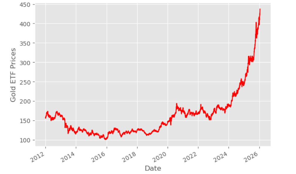
Then, we read the past 14 years of daily Gold ETF price data from a file and store it in Df. This data set includes a date column, which is essential for time series analysis and plotting trends over time. We remove the columns which are not relevant and drop NaN values using dropna() function. Then, we plot the Gold ETF close price.
Output:
Define explanatory variables
An explanatory variable, also known as a feature or independent variable, is used to explain or predict changes in another variable. In this case, it helps predict the next-day price of the Gold ETF.
These are the inputs or predictors we use in a model to forecast the target outcome.
In this strategy, we start with two simple features: the 3-day moving average and the 9-day moving average of the Gold ETF. These moving average serve as smoothed representations of short-term and slightly longer-term trends, helping capture momentum or mean-reversion behavior in prices. Before using these features in modeling, we eliminate any missing values using the .dropna() function to ensure the dataset is clean and ready for analysis. The final feature matrix is stored in X.
However, this is just the beginning of the feature engineering process. You can extend X by incorporating additional variables that might improve the model's predictive power. These may include:
- Technical indicators such as RSI (Relative Strength Index), MACD (Moving Average Convergence Divergence), Bollinger Bands, or ATR (Average True Range).
- Cross-asset features, such as the price or returns of related ETFs like the Gold Miners ETF (GDX) or the Oil ETF (USO), which may influence gold prices through macroeconomic or sector-specific linkages.
- Macroeconomic indicators such as inflation data (CPI), interest rates, and USD index movements can influence gold prices because gold is perceived as a safe-haven asset during times of economic uncertainty.
The process of identifying and constructing such variables is called feature engineering. Separately, selecting the most relevant variables for a model is known as feature selection.
The better your features reflect meaningful patterns in the data, the more accurate your forecasts are likely to be.
Define dependent variable
The dependent variable, also known as the target variable in machine learning, is the outcome we aim to predict. Its value is assumed to be influenced by the explanatory (or independent) variables. In the context of our strategy, the dependent variable is the price of the Gold ETF (GLD) on the following day.
In our dataset, the Close column contains the historical prices of the Gold ETF. This column serves as the target variable because we are building a model to learn patterns from historical features (such as moving averages) and use them to predict future GLD prices. We assign this target series to the variable y, which will be used during model training and evaluation.
To create the target variable, we apply the shift(-1) function to the Close column. This shifts the price data one step backward, making each row's target the next day's closing price. This approach enables the model to use today's features to forecast tomorrow's price.
Clearly defining the target variable is essential for any supervised learning problem, as it shapes the entire modelling objective. In this case, the goal is to forecast future movements in gold prices using relevant financial and economic signals.
Alternatively, instead of predicting the absolute price of gold, we can use gold returns as the target variable. Returns represent the percentage change in gold prices over a specified time period, such as daily, weekly, or monthly intervals.
Non-stationary variables in linear regression
In time series analysis, it's common to work with raw financial data such as stock or commodity prices. However, these price series are typically non-stationary, meaning their statistical properties like mean and variance change over time. This poses a significant challenge because many analytical techniques rely on the assumption that the data behaves consistently. When the data is non-stationary, its underlying structure shifts. Trends evolve, volatility varies, and historical patterns may not hold in the future.
Working with non-stationary data can lead to several problems:
- Spurious Relationships: Variables may appear to be related simply because they share similar trends, not because there's a genuine connection.
- Unstable Insights: Any patterns or relationships identified may not hold over time, as the data’s behaviour continues to evolve.
- Misleading Forecasts: Predictive models built on non-stationary data often struggle to perform reliably in the future.
The core issue is that non-stationary processes do not follow fixed rules. Their dynamic nature makes it difficult to draw conclusions or make predictions that remain valid as conditions change. Before performing any serious analysis, it's crucial to test for stationarity and, if needed, transform the data to stabilize its behaviour.
Two Ways to Work with Non-Stationary Data
Rather than discarding non-stationary variables, there are two reliable strategies to handle them in linear regression models:
1. Make Variables Stationary (Differencing Approach)
One common method is to transform the data to make it stationary. This is often done by focusing on changes in values. For example, price series can be converted into returns or differences. This transformation helps stabilize the mean and reduces trends or seasonality. Once the data is transformed, it becomes more suitable for linear modeling because its statistical properties remain consistent over time.
2. Use Original Non-Stationary Series (Cointegration Approach)
The second strategy allows us to use the original non-stationary series without transformation, provided certain conditions are met. Specifically, it involves checking whether the variables, when combined in a particular way, share a long-term equilibrium relationship. This concept is known as cointegration.
Even if the individual variables are non-stationary, their linear combination might be stationary. If this is the case, the residuals from the regression (the differences between actual and predicted values) remain stable over time. This stability makes the regression valid and meaningful, as it reflects a genuine relationship rather than a statistical coincidence.
In our analysis, we will use this second method by testing for residual stationarity to confirm that the regression setup is appropriate.
Output:
Cointegration p-value between S_3 and next_day_price: 3.1342217460742354e-16
Cointegration p-value between S_9 and next_day_price: 1.268049574487298e-15
S_3 and next_day_price are cointegrated.
S_9 and next_day_price are cointegrated.
The time series S_3 (3-day moving average) and next_day_price, as well as S_9 (9-day moving average) and next_day_price, are cointegrated. Thus, we can proceed with running a linear regression directly without transforming the series to achieve stationarity.
Why You Can Run the Regression Directly?
Cointegration implies that there is a stable, long-term relationship between the two non-stationary series. This means that while the individual series may each contain unit roots (i.e., be non-stationary), their linear combination is stationary and running an Ordinary Least Squares (OLS) regression will not lead to a spurious regression. This is because the residuals of the regression (i.e., the difference between the predicted and actual values) will be stationary.
Key Points to Remember
As cointegration already ensures a valid statistical relationship, making OLS appropriate for estimating the parameters, there is no need to difference the series to make them stationary before running the regression
The regression run between S_3 (or S_9) and next_day_price will capture a valid long-term equilibrium relationship, which cointegration confirms.
Split the data into train and test dataset
In this step, we split the predictors and output data into train and test data. The training data is used to create the linear regression model, by pairing the input with expected output.
Model training is performed on the training dataset, where the model learns from the features and labels.
The test data is used to estimate how well the model has been trained. Comparing different models and evaluating their training time and accuracy is an important part of the model selection process. Model evaluation, including the use of validation sets and cross-validation, ensures the model generalizes well to unseen data.
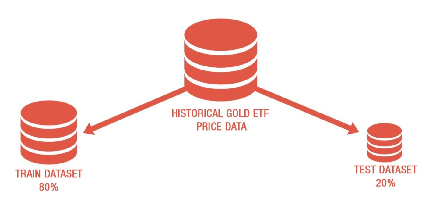
- First 80% of the data is used for training and remaining data for testing
- X_train & y_train are training dataset
- X_test & y_test are test dataset
Create a linear regression model
We will now create a linear regression model. But, what is linear regression?
Linear regression is one of the simplest and most widely used algorithms in machine learning for supervised learning tasks, where the goal is to predict a continuous target variable based on input features. At its core, linear regression captures a mathematical relationship between the independent variables (x) and the dependent variable (y) by fitting a straight line that best describes how changes in x affect the values of y.
When the data is plotted as a scatter plot, linear regression identifies the line that minimizes the difference between the actual values and the predicted values. This fitted line represents the regression equation and is used to make future predictions.
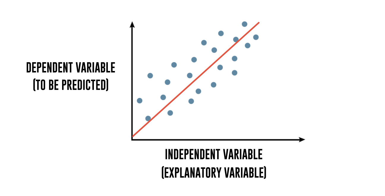
To break it down further, regression explains the variation in a dependent variable in terms of independent variables. The dependent variable - ‘y’ is the variable that you want to predict. The independent variables - ‘x’ are the explanatory variables that you use to predict the dependent variable. The following regression equation describes that relation:
Y = m1 * X1 + m2 * X2 + C
Gold ETF price = m1 * 3 days moving average + m2 * 9 days moving average + c
Then we use the fit method to fit the independent and dependent variables (x’s and y’s) to generate coefficient and constant for regression.
Output:
Linear Regression model
Gold ETF Price (y) = 1.19 * 3 Days Moving Average (x1) + -0.19 * 9 Days Moving Average (x2) + 0.28 (constant)
Predict the Gold ETF prices
Now, it’s time to check if the model works in the test dataset. We predict the Gold ETF prices using the linear model created using the train dataset. The predict method finds the Gold ETF price (y) for the given explanatory variable X.
Output:
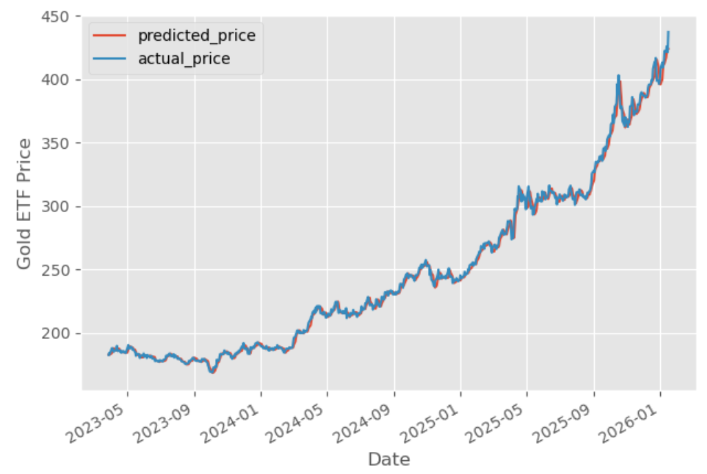
The graph shows the predicted prices and actual prices of the Gold ETF. Comparing predicted prices to actual prices helps evaluate the performance of the trained model and shows how closely the predictions match real-world values. Functions like evaluate_model() can be used to generate diagnostic plots and further evaluate the model's quality.
Now, let’s compute the goodness of the fit using the score() function.
Output:
99.70
As it can be seen, the R-squared of the model is 99.70%. R-squared is always between 0 and 100%. A score close to 100% indicates that the model explains the Gold ETF prices well.
On the surface, this seems impressive. It shows a near-perfect fit between the model's outputs and real market values.
However, translating this predictive accuracy into a profitable trading strategy is not straightforward. In practice, you need to make critical decisions such as:
- When to enter a trade (signal generation)
- How long to hold the position
- When to exit (e.g., based on a predicted reversal or fixed threshold)
- And how to manage risk (e.g., using stop-loss or position sizing)
To illustrate this challenge, we attempted to use predicted prices to generate a simple long-only trading signal.
A position is taken only if the next day's predicted price is higher than today’s closing price. This creates a unidirectional signal with no shorting or hedging. The position is exited (and potentially re-entered) whenever the signal condition is no longer met.
Plotting cumulative returns
Let’s calculate the cumulative returns of this strategy to analyse its performance.
- The steps to calculate the cumulative returns are as follows:
- Generate daily percentage change of gold price
- Shift the daily percentage change ahead by one day to align with our position when there is a signal.
- Create a buy trading signal represented by “1” when the next day's predicted price is more than the current day price. No position is taken otherwise
- Calculate the strategy returns by multiplying the daily percentage change with the trading signal.
- Finally, we will plot the cumulative returns graph
The output is given below:
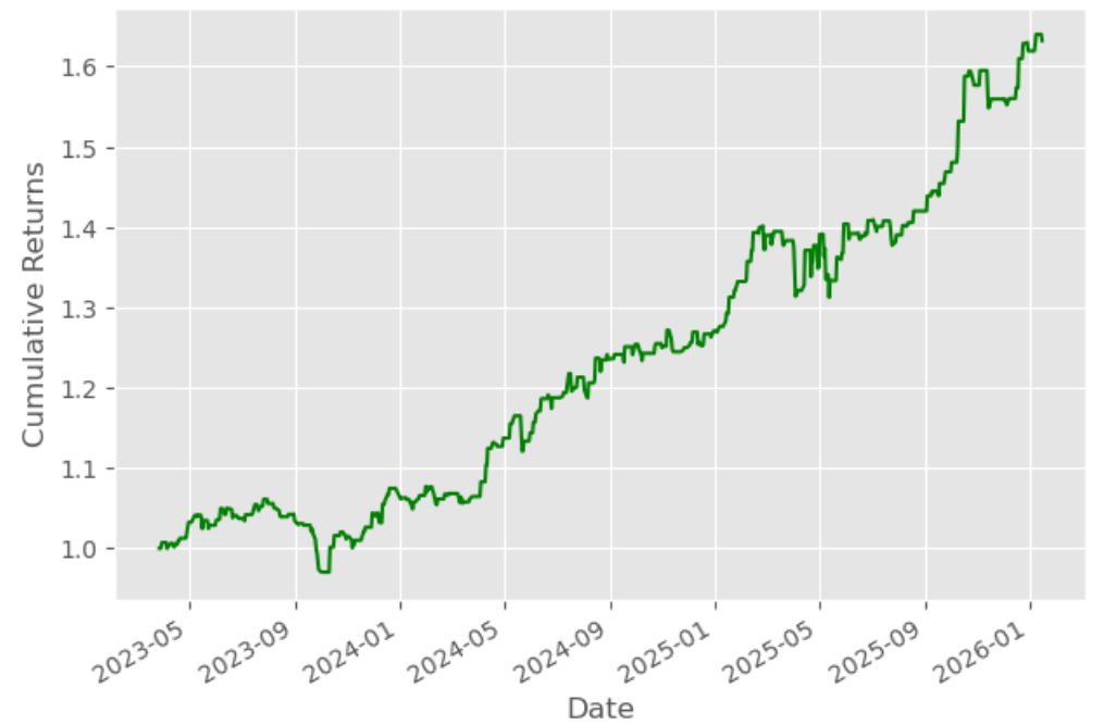
We will also calculate the Sharpe ratio.
The output is given below:
'Sharpe Ratio 1.82'
Given the model’s high predictive accuracy, the Sharpe Ratio of the resulting trading strategy is only 1.82, which is not very good for a scalable and practical trading system.
This disparity highlights a crucial point: good price prediction doesn’t always lead to extremely profitable or risk-adjusted trading performance. Several factors may explain the lower Sharpe Ratio:
The strategy may suffer from unidirectional bias, ignoring shorting or range-bound periods.
- It might not adapt well to market volatility, leading to sharp drawdowns.
- The trading rules are too simplistic, failing to capture timing nuances or noise in the predictions.
In summary, while the model performs well in predicting price levels, converting this into a robust trading strategy requires thoughtful design. Signal logic, timing, position management, and risk controls all play a significant role in enhancing actual strategy performance.
Suggested Reads:
- Top 10 machine learning algorithms which can be used in your trading strategy
- Learn all about Exchange-Traded Funds (ETF)
How to use this model to predict daily moves?
You can use the following code to predict the gold prices and give a trading signal whether we should buy GLD or take no position.
The output is as shown below:
| Date | 2026-01-20 |
|---|---|
| Price | |
| Close | 437.230011 |
| signal | No Position |
| predicted_gold_price | 427.961362 |
Congrats! You've just implemented a simple yet effective machine learning technique using linear regression to forecast gold prices and derive trading signals. You now understand how to:
- Engineer features from raw price data (using moving averages),
- Build and fit a predictive model,
- Use the model for making forward-looking forecasts, and
- Translate those forecasts into actionable signals.
What’s Next?
Linear regression is a great starting point due to its simplicity and interpretability. But in real-world financial modeling, more complex patterns and nonlinear relationships often exist that linear models might not fully capture.
To improve accuracy, you can explore more powerful machine learning regression models, such as:
- Random Forest Regression
- Gradient Boosted Trees (like XGBoost or LightGBM)
- Support Vector Regression (SVR)
- Neural Networks (MLPs for tabular data)
The core structure of your pipeline remains the same: data preprocessing, feature engineering, forecasting, and signal generation. The only change is the model itself. You simply replace the .fit() and .predict() methods with those from your chosen algorithm, possibly adjusting a few additional hyperparameters.
Keep Exploring
Want to dive deeper into using machine learning for trading? Learn step by step how to build your first ML-based trading strategy with our guided course. If you're ready to take it to the next level, explore our Learning Track. Experts like Dr. Ernest Chan will guide you through the entire lifecycle, from idea generation and backtesting to live deployment, using advanced machine learning techniques.
File in the download:
Gold Price Prediction Strategy - Python Notebook
Disclaimer: All investments and trading in the stock market involve risk. Any decisions to place trades in the financial markets, including trading in stock or options or other financial instruments is a personal decision that should only be made after thorough research, including a personal risk and financial assessment and the engagement of professional assistance to the extent you believe necessary. The trading strategies or related information mentioned in this article is for informational purposes only.
