Modelling Asymmetric Volatility with the GJR-GARCH Framework

By Manusha Rao

You may have noticed that markets sometimes remain calm for weeks and then swing wildly for a few days. That’s volatility in action. It measures how much prices move—and it’s a big deal in trading and investing because it reflects risk. But here’s the catch: estimating volatility isn't straightforward.

A 2% drop often sparks more headlines than a 2% gain. That’s asymmetric volatility—and it's what traditional models miss.

Enter the GJR-GARCH model!

Prerequisites

This blog focuses on volatility forecasting using the GJR-GARCH model, with a practical Python implementation based on the NIFTY 50 index. It explains the concept of asymmetric volatility, how it differs from the traditional GARCH model, and provides tools for evaluating forecast quality through visualizations and diagnostics.

To understand and apply the GJR-GARCH model effectively, it's important to start with the basics of time series analysis. Begin with Introduction to Time Series to get familiar with trend, seasonality, and autocorrelation. If you're exploring how deep learning compares to traditional models, read Time Series vs LSTM Models for a conceptual comparison.

Since GARCH and GJR-GARCH models rely on stationary time series, study Stationarity to learn how to prepare your data. Enhance this knowledge by reading The Hurst Exponent for insights into long-term memory in time series and Mean Reversion in Time Series for understanding mean-reverting behavior—often linked with volatility clusters.

You should also be familiar with the ARMA family of models, which are foundational to ARIMA and GARCH. For this, refer to the ARMA Model Guide and its companion blog ARMA Implementation in Python. Lastly, to grasp the terminology and concept behind GARCH, the Quantra glossary entries on GARCH and Volatility Forecasting using GARCH are essential resources.

In this blog, we will explore the following:

• Difference between GARCH and GJR-GARCH models
• A brief look at the GARCH model
• Introduction to the GJR-GARCH model
• Volatility Forecasting on NIFTY 50 Using GJR-GARCH in Python

Difference between GARCH and GJR-GARCH models

The GARCH model captures volatility clustering but assumes that positive and negative shocks have a symmetric effect on future volatility. In contrast, the GJR-GARCH model accounts for asymmetry by giving more weight to negative shocks, which reflects the leverage effect commonly observed in financial markets. Why? Because fear drives faster and stronger reactions than optimism in financial markets.

GJR-GARCH introduces an additional parameter that activates when past returns are negative. This makes it more suitable for modelling real-world stock data, where bad news typically causes higher volatility.

For example, during the COVID-19 market crash in March 2020, the NIFTY 50 saw sharp declines and sudden spikes in volatility driven by panic selling shown below.

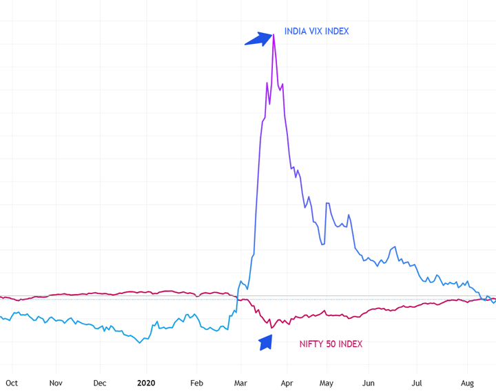
Source: TradingView

A GARCH model would understate this asymmetry, while GJR-GARCH captures the heightened volatility following negative shocks more accurately. Overall, GJR-GARCH is a more flexible and realistic extension of the standard GARCH model.

A brief look at the GARCH model

The GARCH (Generalized Autoregressive Conditional Heteroskedasticity) model is a popular statistical tool for forecasting financial market volatility. Developed by Tim Bollerslev in 1986 as an extension of the ARCH model, GARCH captures the tendency of volatility to cluster over time—meaning periods of high volatility tend to be followed by periods of high volatility, and periods of calm are followed by more periods of calm.

In essence, the GARCH model assumes that today’s volatility depends not only on past squared returns (as in ARCH) but also on past volatility estimates. This makes it especially useful for modelling time series data with changing variance, such as asset returns.

The general equation for a GARCH(p, q) model, which models conditional variance, is:

• σ²_t: Represents the conditional variance of the time series at time 't'.
• ω: A constant term representing the long-run or average variance.
• Σ(α_i * ε²_t−i): The ARCH component, capturing the effect of past squared errors on the current variance.
• Σ(β_j * σ²_t−j): The GARCH component, capturing the effect of past conditional variances on the current variance.

Note: GARCH(1,1) is the simplest form of the GARCH model:

σ²_t = ω + α₁ ε²_t−1 + β₁ σ²_t−1

With only three parameters (constant, ARCH term, and GARCH term), it's easy to estimate and interpret—ideal for financial data where too many parameters can be unstable.

Introduction to the GJR-GARCH model

The GJR-GARCH model, proposed by Glosten, Jagannathan, and Runkle (1993), is an extension of the standard GARCH model designed to capture the asymmetric effects of news on volatility.

The GJR-GARCH(1,1) formula is given by:

σ²_t = ω + α₁ ε²_t−1 + γ ε²_t−1 I_t−1 + β₁ σ²_t−1

Now that we understand the GJR-GARCH model formula and its intuition, let’s implement it in Python. We’ll use the arch package, which offers a simple yet powerful interface to specify and estimate GARCH-family models. Using historical NIFTY 50 returns data, we’ll fit a GJR-GARCH(1,1) model, generate rolling volatility forecasts, and evaluate how well the model captures market behavior, especially during turbulent periods.

Volatility Forecasting on NIFTY 50 Using GJR-GARCH in Python

Step 1: Import the necessary libraries

The tqdm library is used to show a progress bar when your code is doing something that takes time — like running a loop with a lot of steps.

It helps you see how much is done and how much is left, so you don’t have to guess if your code is still running or stuck.

Step 2: Download NIFTY50 data

Here we are using NIFTY 50 data from 2020 to 2025.

Next, calculate the daily log returns and express in percentage terms. Models like GARCH work better when the input numbers are not too tiny (like 0.0012), as very small values can make it harder for the optimizer to converge during model fitting.

Step 3: Specify the GJR-GARCH model

To model a GJR-GARCH model in Python,the arch package is used. Use Student's t-distribution for residuals, which captures fat tails often observed in financial returns. Feel free to use the distribution that best suits your trading needs or data distribution.

Here,

p = 1

Number of lags of past squared returns (ARCH term)

o = 1

Number of lags for asymmetry term – this enables the GJR-GARCH (or GARCH with leverage effect)

q = 1

Number of lags of past variances (GARCH term)

Step 4: Fit the model

The output is as follows:

• The ARCH term (alpha[1]), which measures the impact of past shocks, is significant at the 5% level, though relatively small (0.0123).
• The GARCH term (beta[1]) is high at 0.9052, implying that volatility is highly persistent over time.
• The leverage effect (gamma[1] = 0.1330) is significant, confirming the presence of asymmetry—negative shocks increase volatility more than positive ones, a common feature in equity market data.
• The estimated degrees of freedom (nu = 7.6) for the Student's t-distribution suggest the data exhibits fat tails, justifying the choice of this distribution to capture extreme returns more accurately.

Step 5: Residual diagnostics

This block of code is for residual diagnostics after fitting your GJR-GARCH model. It helps you visually assess how well the model has captured volatility dynamics.

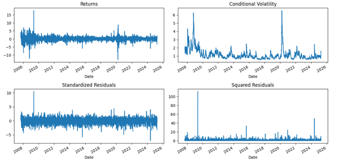
The GJR-GARCH model performs well in capturing volatility dynamics during major market events, especially periods of financial distress. Notable spikes in conditional volatility are observed during the 2008 global financial crisis and the 2020 COVID-19 pandemic. The asymmetry component (gamma) plays a key role here, amplifying volatility predictions in response to negative returns—mirroring real-world investor behavior where fear and bad news drive sharper market reactions than optimism.

Step 6: Make rolling forecasts of volatility

A more practical approach to forecast volatility is to make one-step-ahead predictions using information available up to time t, and then update the model in real time as each new data point becomes available (i.e., as t progresses to t+1, t+2, etc.). In simple terms, each day we incorporate the latest observed return to forecast the next day's volatility.

Here we take train the model on 500 days of past returns, to forecast 1-day ahead volatility, repeated daily.

Now you would want to compare GARCH's 1-day forecast to some observable actual volatility.

The usual method is to compute realized daily volatility as a rolling standard deviation.

However, if you're forecasting for 1 day, the realized volatility you should ideally compare it to is:

the actual return (i.e., squared return of the next day), or a smoothed proxy like a 5-day rolling standard deviation (if you want to remove noise).

As illustrated in the plot below, periods of elevated market uncertainty, such as mid-2024, exhibit significant spikes in the 1-day ahead forecasted volatility, reflecting heightened risk perception. Conversely, calmer periods like early 2023 show reduced volatility expectations. This approach enables traders and risk managers to adaptively adjust exposure and hedging strategies in response to anticipated market conditions.

The GJR-GARCH model proves especially valuable for its ability to react sensitively to downside shocks. It is a robust tool for short-term volatility forecasting in index-level data like the NIFTY 50 or stock data.

Now let us check the correlation between the realized and forecasted volatility.

Output:

Correlation between Forecasted and Realized Volatility: 0.7443

The observed correlation of 0.74 between the 5-day rolling realized volatility and the GJR-GARCH forecasted volatility indicates that the model effectively captures the dynamics of market volatility.

Specifically, the GJR-GARCH model, which accounts for asymmetric responses to positive and negative shocks (i.e., volatility reacts more to negative news), aligns well with the actual realized volatility. A strong correlation like this suggests that the model can forecast periods of high or low volatility in a directionally accurate way.

Conclusion

Market volatility isn’t just numbers—it reflects human psychology. The GJR-GARCH model goes a step beyond traditional volatility estimators by recognizing that fear has a stronger market impact than optimism. By modelling this behaviour explicitly, it provides a more accurate and behaviourally sound way to forecast volatility in various assets.

Next Steps

Once you're comfortable with the GARCH family, you can move on to more complex volatility modeling techniques. A good next read is Time-Varying-Parameter VAR (TVP-VAR), which introduces models that handle stochastic volatility and structural changes over time.

You can also explore ARFIMA models for handling long-memory processes, which are common in financial market volatility. Understanding these models will help you create more robust, adaptable forecasting systems.

To develop effective trading strategies, go beyond modeling. Combine your GJR-GARCH insights with practical methods from Technical Analysis to detect trends and momentum, use Trading Risk Management to protect against losses, explore Pairs Trading for market-neutral strategies, and understand Market Microstructure to account for execution and liquidity dynamics.

Finally, for a structured and comprehensive journey into algorithmic trading, consider enrolling in the Executive Programme in Algorithmic Trading (EPAT). EPAT covers advanced topics such as stationarity, ACF/PACF, ARIMA, ARCH, GARCH, and more, with practical training in Python strategy development, statistical arbitrage, and alternate data. It’s the perfect next step for those ready to apply their quantitative skills in real markets.

File in the download:

GJR GARCH Python Notebook

Login to Download

Disclaimer: All investments and trading in the stock market involve risk. Any decision to place trades in the financial markets, including trading in stock or options or other financial instruments is a personal decision that should only be made after thorough research, including a personal risk and financial assessment and the engagement of professional assistance to the extent you believe necessary. The trading strategies or related information mentioned in this article is for informational purposes only.